Align the Design: Considering and Evaluating Target-Date Glide Paths

Defining the objective
In our most recent survey, consultants said that the glide path (or the way a target-date strategy changes over time) is the key factor in evaluating default options, or Qualified Default Investment Alternatives (QDIAs). Further, they suggested that the primary objective of glide paths should be to “maximize asset returns while minimizing volatility relative to the retirement liability.”

PIMCO agrees with these views. The majority of U.S. workers will look to their DC plan to replace 30% or more of their pre-retirement income. In our view, the likelihood of achieving this goal should be the measure by which plan fiduciaries select and evaluate QDIAs. Other considerations, including expected returns, volatility, value at risk and more, may then follow.

Achieving these goals is vital not only to workers but employers, too. Delayed retirement may lead to lower productivity, delay and frustrate younger workers seeking to advance and add to employer costs for both healthcare and compensation.

Defining the retirement income liability: looking back
The first step in evaluating a QDIA is defining the need for retirement income. This can be understood as the present value of the stream of cash flows that a person will need in retirement. A common approach is to consider the cost of buying a lifetime income stream via an immediate annuity. For example, consider a 65-year-old male who has accumulated $400,000 in DC assets. This is a substantial sum, but is it enough to deliver an adequate income in retirement? One way to answer the question is to look at the income that could be delivered with an annuity. Based on average annuity quotes between March 2013 and March 2015 (Figure 1), he may have received an annuity payout equal to a 6.5% to 7.2% return, providing an annual income of $25,899 to $28,665 a year. If we assume his final pay was $75,000, his income replacement rate would be 35% to 38%, depending on the year he retired.

But what if he wanted to purchase a real annuity in which the payout is adjusted annually consistent with CPI? Real annuity quotes have averaged 71% of the nominal payout. This means the dollars paid would have delivered $17,885 to $20,501 a year, or 4.5% to 5.1% annually, in real terms. His real income replacement rate would equal 24% to 27% of his final salary.

Depending on the inflation rate, we can determine whether the nominal annuity or the real annuity was a better deal. With 3% inflation, the retiree’s breakeven would come at age 77 – but at 4% it would be age 74. Despite a lower initial payout, the real annuity would likely be the better bet as it would minimize inflation risk.

To evaluate a QDIA structure, we can look at the income stream the investment would have allowed the retiree to purchase relative to his ending salary. This analysis will show us how well the structure has performed relative to the goal. If the goal was to replace 30% of income at retirement, then our sample retiree fails by 3–6 percentage points in real terms.

Defining the liability: looking forward
To look forward, we need to gauge the progress an individual has made in accumulating DC savings relative to their retirement income needs. One way would be to consider the QDIA’s probability of success based on future real annuity prices – which, unfortunately, do not exist. Thus, we have identified a proxy for future annuity rates. We have found that a 20-year ladder of zero-coupon TIPS (Treasury Inflation-Protected Securities)¹ provides the best available proxy for annuity rates. If we compare real annuity rates to the TIPS ladder, we see a 94% correlation and a small difference in the payout rate (Figure 2).

Using the TIPS ladder, we can look to the likely real future cost of retirement by considering current and forward prices of TIPS. This approach allows us to evaluate glide paths relative to a retirement income objective. It also points to the asset type that best matches – and thus reduces – risk relative to the liability, i.e., the TIPS ladder.

Retirement income matching asset: TIPS
To reduce risk relative to liabilities, DC plans – like their defined benefit (DB) cousins – should seek assets that are liability-aware. For DC plans, that asset is TIPS. Using the TIPS ladder as the retirement income stream “liability,”² we can evaluate both assets and glide paths. If we look at asset classes, we can determine which ones correlate best to the liability. Figure 3 shows a low correlation of 0.1 between the monthly returns of the S&P 500 Index and the retirement liability. In contrast, Figure 4 shows the correlation between the retirement liability and long TIPS is very tight (0.95).

In Figure 5, we show the absolute risk (volatility) side-by-side with the risk relative to retirement income generated by the TIPS ladder. This illustrates the reduced retirement income risk of long TIPS compared to stocks, nominal bonds and even cash.

Evaluating glide paths
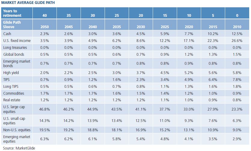
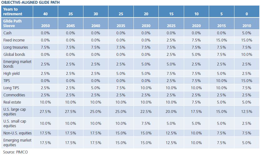
By aligning the target-date design to the retirement liability, DC participants have a higher likelihood of meeting their income goals. Let’s consider two glide paths: the Market Average Glide Path³ and an Objective-Aligned Glide Path, as shown in Figure 6.

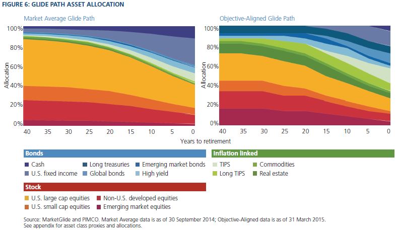
The Objective-Aligned Glide Path has a greater proportion of assets allocated to TIPS, including a 2.5%–10.0% allocation to long duration TIPS. Back-tested results from January 2004 to March 2015 (see Figure 7) show that the Objective-Aligned Glide Path has a much tighter correlation to the retirement liability than the Market Average Glide Path.

According to back-tested results from February 2004 to March 2015, the reduced tracking error (relative to the retirement liability) for the Objective-Aligned Glide Path does not come at the expense of investment returns. As Figure 8 shows, the simulated excess returns (relative to 3-month T-bills) for the Objective-Aligned Glide Path are in line with, or even higher than, those of the Market Average Glide Path across vintages. The Objective-Aligned Glide Path has a higher ratio of excess return to tracking error than the Market Average Glide Path.

Our back tests also show that the Objective-Aligned Glide Path yields greater inflation-adjusted capital appreciation. For instance, assume participants started with $350,000 and invested in the Market Average Glide Path and the objective-Aligned Glide Path at age 55 (from January 2004 through March 2015 ⁴). Figure 9 shows that the accumulated real balance is $48,624, or 7% higher, for the Objective-Aligned Glide Path compared with the Market Average Glide Path.

Reduced risk of failure: Looking forward
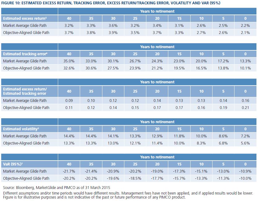
Notably, despite the reduced risk, the return expectations⁵ for the two glide paths are similar. While the Objective-Aligned Glide Path has lower estimated tracking error⁶, VaR (95%)⁷ and other risk statistics, Figure 10 shows that it has a higher ratio of excess return to tracking error across vintages than the Market Average Glide Path.

By aligning the asset allocation to the retirement income liability, the probability of achieving at least a 30% income replacement goal⁸ increases by almost 5 percentage points for the Objective-Aligned Glide Path compared with the Market Average Glide Path (see Figure 11).

Meeting real objectives
Plan sponsors confront a host of fiduciary responsibilities, but among the most important is selecting and evaluating a QDIA glide path that will best maximize the probability that their participants will retire both on time and with sufficient lifetime income. This defines the DC-plan objective, in short, to maximize asset returns while minimizing volatility relative to the retirement liability. Participants are more apt to meet this objective when the liability is defined as a lifetime income stream and the selected glide path keeps pace with this liability. The Objective-Aligned Glide Path has the potential to improve the probability of a participant having the real retirement income they need – which is the true goal of both employees and employers.

We will explore this further in our next DC Design, which will focus on DC retirement liability benchmarking.

– Sebastien Page and Steve Sapra contributed to this article.

Appendix:

¹ The zero-coupon U.S. TIPS yield curve was constructed by Haver Analytics.

² To evaluate the TIPS ladder “liability” cost we calculated the historical present value of a 20-year zero-coupon TIPS ladder using the TIPS yield curve provided by Haver Analytics. For example, if they need $50,000 annually, the cost to buy that income stream is $902,094 in 2013 and they need $936,051 in 2014.

³ The Market Average Glide Path is constructed by MarketGlide and is an average of the 40 largest target-date strategies in the market.

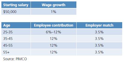
⁴ Starting salary at age 25: $50,000; real wage growth rate: 1%; participant savings rate from age 55 and older is 12%; the employer match rate is 3.5%.

⁵ Estimated returns and volatilities for assets are simulated as outlined below. This long-horizon simulation process was detailed in “Rethinking Retirement Risk,” by Niels Pedersen (December 2014). See /EN/Insights/Pages/Rethinking-Retirement-Risk.aspx.

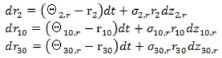
• The simulation of nominal yield curves follows a three-factor model Cox-Ingersoll-Ross (CIR) process
  
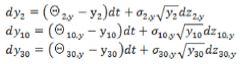
• The simulation of real yield curves follows a reduced form three-factor Vasicek model
  
• The term structure of break-even inflation is defined by the difference between the term structure of nominal and real rates.
  
  
• Realized inflation in a given year is simulated as break-even inflation plus a stochastic term.
  
  
• Long-horizon risky asset returns use a parsimonious specification of returns that builds the expected return as a risk-free rate plus a risk premium.

⁶ Tracking error is calculated as the standard deviation of the difference between simulated asset returns and the change in retirement liability. The discounted present value of the 20-year liability stream is calculated using the simulated real yield curves as noted above.

⁷ Value-at-risk (VaR) is an estimate of the minimum expected loss at a desired level of significance over a 12-month horizon.

⁸ The income replacement rate was calculated using the above long-horizon assets simulation process and the following DC assumptions. The simulated 10-year real rate was used as a proxy for the real annuity rate in the calculation of the income replacement rate. The distribution of the income replacement rate was plotted from results of a simulation of 5,000 trials; the probability of achieving at least a 30% income replacement rate was derived from the distribution. Additional assumptions:

Asset class proxies:
U.S. Large Cap: S&P 500 Index; U.S. Small Cap: Russell 2000 Index; Non-U.S. Equities: MSCI EAFE Total Return, Net Div Index; EM Equity: MSCI EM Index; Real Estate: Dow Jones U.S. Select REIT TR Index; Commodities: Bloomberg Commodity Index; High Yield: BofA Merrill Lynch U.S. High Yield, BB-B Rated, Constrained Index; Emerging Market Bonds: JPMorgan Government Bond Index - Emerging Markets Global Diversified (Unhedged); Global Bonds: JPMorgan GBI Global Index (USD Hedged); Fixed Income: Barclays U.S. Aggregate Index; TIPS: Barclays U.S. TIPS Index; Long Treasuries: Barclays Long-Term Treasury Index; Long TIPS: Barclays U.S. TIPS: 10 Year+ Index; Cash: BofA Merrill Lynch 3-Month Treasury Bill Index.

Glidepath Allocations:

References:
Niels K. Pedersen, “Rethinking Retirement Risk,” December 2014. /EN/Insights/Pages/Rethinking-Retirement-Risk.aspx

Bransby Whitton and Klaus Thuerbach, "Using a Real Liability to Assess Retirement Readiness and Inform Investment Decisions," June 2014.
/EN/Insights/Pages/Using-a-Real-Liability-to-Assess-Retirement-Readiness-and-Inform-Investment-Decisions.aspx