- Four of the world’s major central banks are now “all in” when it comes to ballooning their balance sheets in correlated, if not coordinated, efforts to achieve escape velocity in their economies.
- In accounting for the impact of quantitative easing on two key balance sheets, we are able to interpret, monitor and calibrate the programs currently in place. This in turn can help us prepare portfolios if – or when – sentiments and inflation expectations shift.
“It is sometimes better to study a balance sheet than it is to believe a model”
Rudiger Dornbusch, 1980
With the Bank of Japan’s recent “shock and awe” decision to double down on quantitative easing (QE), four of the world’s major central banks – the BOJ, the Fed, the Bank of England and the Swiss National Bank – are now “all in” when it comes to ballooning their balance sheets in correlated, if not coordinated, efforts to achieve escape velocity in their economies.
These programs are enormous and untested, and they risk serious unintended consequences even if they ultimately succeed in reflating these economies. QE is controversial, but it’s also not well or widely understood – primarily because there is no agreed upon model for how it works. And theoretical economic models themselves can sometimes get in the way, obfuscating instead of illuminating.
Still, it can be worthwhile to
account for QE even if it may be difficult to model it. In accounting for QE’s impact on two key balance sheets – those of a country’s central bank and its commercial banking system – as well as the relationship between them and nominal gross domestic product (GDP), we are able to
interpret,
monitorandcalibrate the QE programs currently in place. And as these programs continue, this framework should be able to provide a more or less real-time signal and explanation for why these programs are succeeding (or failing).
Two key ratios
We begin with two key ratios that are essential to accounting for QE.
In monetary economics, the “
Cambridge k ” ratio is the ratio of the broad money supply – currency plus the checkable and time deposit liabilities of the commercial banking system – to nominal GDP. It is a concept that was developed by John Maynard Keynes and others, who tried to understand – and, yes, model – it in the 1920s. Later, in
The General Theory of Employment, Interest and Money, Keynes developed a
theory of liquidity preference, which hypothesized that over a business or credit cycle
k would depend inversely on the rate of interest on “bonds.” But Keynes also argued that the demand for money – and thus
k – would depend on a precautionary motive or in certain circumstances (deflation) a speculative motive to hold money. He argued that in slumps
k is not constant or even mean-reverting but rises with the demand for safe assets. Note that in an open economy there can be a global precautionary demand for the money supply of a safe haven or reserve currency so that
k can and does fluctuate (a lot) with global risk appetite. This makes it much harder for central banks to model and predict money demand in the real world than in the textbooks.
The “money multiplier” reflects the endogenous creation of broad money by the banking system. It is pro cyclical: In slumps, banks would rather keep reserves at the central bank than lend them out. As they do so, credit creation falls. Note that the central bank controls B (the size of its balance sheet) directly, but it can only influence the money multiplier – and thus the stock of broad money – indirectly though monetary policy. This slippage between the levers of monetary policy and the supply of broad money is especially acute when, as is the case in all four QE economies, banks want to keep enormous excess reserves on deposit at the central bank at rates far lower than they could earn on extending new loans.
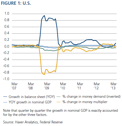
Nominal GDP growth can always be accounted for by the growth in the central bank balance sheet, the observed change in demand for broad money and the observed change in the money multiplier.
%∆nominal GDP ≡ %∆P + %∆Y ≡ %∆B + %∆x - %∆k
Note that this equation is an identity, not a theory or model of how changes in the central bank balance sheet influence nominal GDP growth. However it
can be used to
interpret,
monitor and calibrate any observed slippage between the growth in the balance sheet and the growth in nominal GDP in terms of observed shifts in money demand and the money multiplier. And for this reason it is quite useful. Moreover,
any theory or model of QE must be consistent with the above relationship between the balance sheet, the money multiplier (credit creation) and money demand.
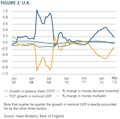
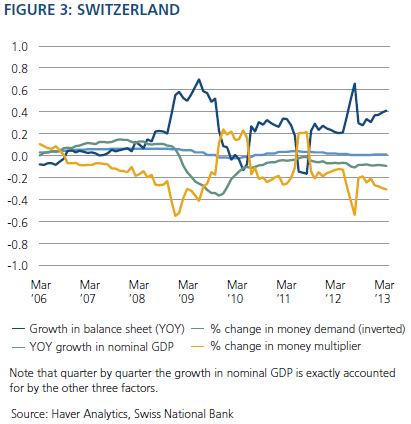
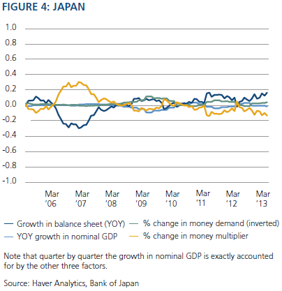
The QE parade in pictures
The following four charts (all drawn to the same scale) each apply this framework to the Fed, BOE, BOJ and SNB. QE supporters look at these charts and see an endogenous and, to date, justified response by central banks to a largely exogenous collapse in the money multiplier (commercial banks in the bunker hoarding reserve deposits at the central bank instead of extending credit to the private sector) and a surge in the public’s desire to rebalance portfolios in favor of money at the expense of holding fewer risky assets. And of course the rise in balance sheets, while huge, has not been sufficient to restore nominal GDP growth to its old normal pace. According to this view, had QE been excessive, nominal GDP would have surged, and of course it hasn’t.
QE detractors look at these same charts and see something quite different. They see QE as not responding to the collapse in the money multiplier but to some extent
causing it. In this account QE – and the flatter yield curves that have resulted from it – has itself broken the monetary transmission mechanism, resulting in central banks pushing ever more liquidity on a limper and limper string. In this view, it is not inflation that’s at risk from QE, but rather, the health of the financial system. In this view, instead of central banks waiting for the money multiplier to rebound to old normal levels before QE is tapered or ended, central banks must taper or end QE first to induce the money multiplier and bank lending to increase.
What are the limits to balance sheet expansion?
Recall from our accounting relationships we can always write:
Thus if there are limits to balance sheet expansion, that is equivalent to saying there is a limit to the ratio of money demand to the money multiplier. We have just discussed two opposing views of QE and the money multiplier x. While there is disagreement about the causes of the fall in the money multiplier, all would agree that a rebound in the money multiplier and in bank lending – for whatever reason – would be a positive indicator of the healing of these major financial systems. And note from the above equation it would tend to reduce the size of the balance sheet relative to GDP by boosting the denominator.
There is much less disagreement about what has happened to money demand under QE. Money demand
k has been boosted in these countries by the Keynesian precautionary demand motive and as well for the U.S., Japan and Switzerland by
global safe haven/flight-to-quality capital inflows. Note that this effect is especially evident in the Switzerland chart. A fall in money demand due to a normalization of global risk appetite and/or expectations of rising inflation would limit balance sheet expansion in these countries by reducing the demand for money. However, also note:
The SNB and BOJ want more inflation and the Fed and the BOE are within some range willing to tolerate it. Finally, a weaker currency in any of these countries could also limit balance sheet expansion by reducing the demand for money, but it is well to remember that as all four of these countries are now doing some form of QE (or in the case of the U.K., is poised to resume as necessary), the net impact on exchange rates among the four to some extent cancels out.
The bottom line
I find this framework useful for organizing my thinking about the relationship between QE and nominal GDP growth, and I hope you do too. The era of QE will finally come to an end when these programs ultimately succeed – or fail, with the costs overwhelming the benefits.
While I have focused on the experience of individual countries, there are potential global externalities, benefits and costs to QE that are also important. As of now, commodity prices and the price of gold do not suggest that markets are worried about the global inflation consequences of QE. But only two years ago, when there was trillions less of QE in the global financial system, they were. This reminds us that sentiment and inflation expectations can shift. If and when they do, the exit dynamics from this very crowded global QE trade will likely be more complex than they may appear: nasty and brutish for those who are short.
Past performance is not a guarantee or a reliable indicator of future results. All investments contain risk and may lose value. This material contains the opinions of the author but not necessarily those of PIMCO and such opinions are subject to change without notice. This material has been distributed for informational purposes only and should not be considered as investment advice or a recommendation of any particular security, strategy or investment product. Information contained herein has been obtained from sources believed to be reliable, but not guaranteed. No part of this material may be reproduced in any form, or referred to in any other publication, without express written permission. PIMCO and YOUR GLOBAL INVESTMENT AUTHORITY are trademarks or registered trademarks of Allianz Asset Management of America L.P. and Pacific Investment Management Company LLC, respectively, in the United States and throughout the world. © 2013, PIMCO.
© PIMCO
www.pimco.com
© PIMCO
Read more commentaries by PIMCO