Stress Testing Portfolio Risk Estimates

The three-year historical volatility closely matches the IV across the equity asset classes, but this has not always been the case. There is close agreement between RA and the IV for developed international (EFA) and emerging markets (EEM). International equity allocations should not be very sensitive to which risk estimates are used. The domestic equity asset classes exhibit larger differences between RA and IV, but the trailing volatility and IV are very close. Research Affiliates Asset Allocation Interaction indicates that the risk and return metrics are for a 10-year outlook. The IV is for the next 1.3 years (the options expire on January 20, 2023).

The options market reflects current economic conditions and the near-term outlook, as opposed to the longer view from RA. I acknowledge that long-term estimates of volatility may not be useful for short-term forecasting. Practitioners should realize that just like with returns, which will be higher or lower (within a decade) than the overall average across the decade, the same can be true for volatility.

Looking at the table of expected returns, with volatilities from three sources, it is not obvious whether the differences in volatility are materially significant.

To calculate portfolio risk, I use correlations between the ETFs calculated using monthly returns for the past three years (calculated by PortfolioVisualizer.com). In practice, the correlations between asset classes vary with the time horizon, and the correlations change over time. The correlations between the ETFs using three years of monthly data are somewhat higher than the correlations between annual returns over the past 16+ years (the maximum number of years of history for EEM, the shortest-lived of the ETFs). The correlation matrix values are in the Appendix. The average correlation between the equity asset classes using month returns is 87%, as compared to 80% using annual returns. The average correlation among all six asset class ETFs is 25% using monthly data and 21% using annual data.

Analysis

For this calculation, I am assuming normally distributed returns. The probability of having a loss of two standard deviations or more is 2.3%, or 1-in-44. Since we are looking at estimates of annual returns, a two-standard-deviation (2SD) loss is approximately a twice-in-a-lifetime event. In the historical record, large market losses occur more frequently than the normal distribution suggests, but the assumption of normality provides a reasonable basis for thinking about potential loss.

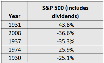
Using RA’s expected return and volatility for the S&P 500, a 2SD 12-month loss would be -26% (4.9%-2*15.5%). Using the IV or three-year volatility for the S&P 500 with RA’s expected return, a 2SD loss would be -33%. In NYU-Stern’s historical stock market returns back to 1928 (93 years), the S&P 500’s 2SD annual loss was -27%. There are five calendar years in the 93-year period with returns of -25% or worse. These results give a sense that the estimated extreme losses using either IV or RA parameters are in line with history for the S&P 500.

Five worst years for the S&P 500 over the past 93 years (Source: NYU-Stern)

The sensitivity of portfolio loss potential to the choice of risk input (RA, IV, or historical volatility) depends on the specific asset allocation, so I have generated several example portfolios.

Example 1

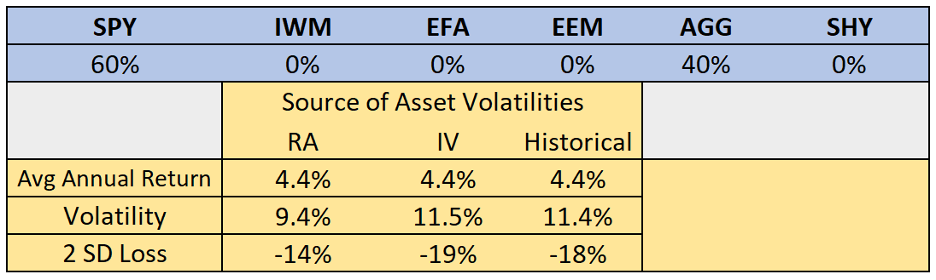
Risk and return for the 60% S&P 500 / 40% Aggregate Bond portfolio using RA volatilities, IV, and historical volatility

For the benchmark 60% S&P 500 / 40% allocation, the expected portfolio volatility calculated using IV or historical volatility is about 20% greater than the portfolio calculated using RA’s outlook for asset volatilities. The estimated 12-month 2SD loss using RA inputs is -14%, versus -19% using IV and -18% using historical volatility.

To put the differences in portfolio risk in context, I have calculated what the equity allocation would be to increase the estimated volatility using RA inputs to match that of the 60/40 allocation using IV.

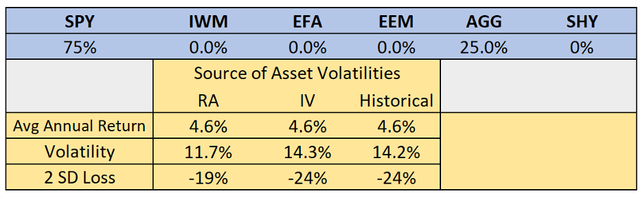
Risk and return for the 75% S&P 500 / 25% Aggregate Bond portfolio using RA volatilities, IV, and historical volatility

The estimated volatility of a 75% S&P 500 / 25% Aggregate Bond portfolio using RA inputs matches that of the 60/40 portfolio using IV. The difference in estimated portfolio risk level from using RA inputs versus IV is equivalent to the risk difference between a 60% SPY / 40% AGG portfolio and a 75% SPY / 25% AGG portfolio.

In 2008, a 60% SPY / 40% AGG portfolio had a return of -19.0% as compared to -25.7% for the 75% SPY / 25% AGG portfolio. The magnitude of the 2SD loss for the 60/40 portfolio calculated using the Ivs is very close to the 2008 losses.

Example 2

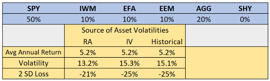
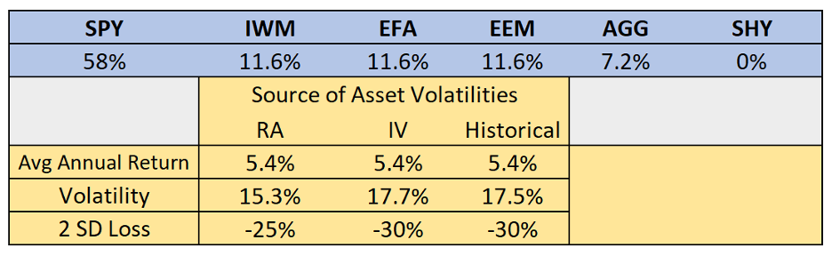
As a second example, I chose an 80% equity portfolio with 10% allocation to small-cap stocks (IWM), 10% to developed international stocks, and 10% to emerging market stocks.

Risk and return for the allocation in the top row using RA volatilities, IV, and historical volatility

The estimated portfolio risk levels using IV and three-year historical volatility are very similar, but estimated risk is significantly lower using RA’s volatility estimates. To estimate the effective difference in portfolio risk levels using the different inputs, I proportionately raised the equity allocations and reduced the bond allocation to bring the portfolio volatility calculated using RA inputs in line with the baseline results using IV (see table below).

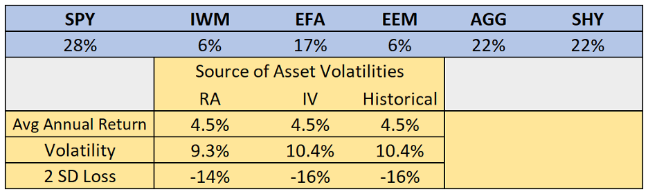
Risk and return for the allocation in the top row using RA volatilities, IV, and historical volatility

Reducing the bond allocation from 20% to 7.2% and raising the allocations to each of the equity ETFs proportionately brings the 2SD loss using RA inputs to -25%, matching the 2SD loss using IV and historical volatilities for the 80% equity / 20% bond portfolio. The difference in risk between using the RA volatilities versus either IV or historical volatility is equivalent to the difference between the 80% equity portfolio and a 92.8% equity portfolio.

The 2008 return for the original portfolio, with 20% bonds, was -29.2%, as compared to -35.2% for the portfolio with 7.2% bonds.

Example 3

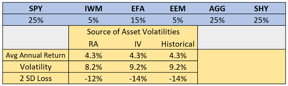
For the third example, I chose a portfolio with a 50% bond allocation. As noted, I am using the RA inputs for fixed income volatility for the IV risk analysis because of the lack of longer-dated options on AGG and SHY. For this reason, the risk estimates using RA inputs and IV will be much closer. The historical volatilities for SHY and AGG are close to the RA estimates, as well, so the results would not change much using the historical values.

Risk and return for the allocation in the top row using RA volatilities, IV, and historical volatility

As in the previous examples, the estimated portfolio risk level estimated using RA inputs is below those using IV and historical volatility. Using the RA inputs, the fixed income allocation would need to be lowered from 50% to 44% (and proportionately raised for each equity ETF) to match the baseline risk level calculated using IV and historical volatility (see table below).

Risk and return for the allocation in the top row using RA volatilities, IV, and historical volatility.

The baseline allocation, with 50% equities, had a 2008 return of -15.8% vs. -18.9% for the modified case with 56% equity.

Discussion

The differences in estimated portfolio risk from using RA’s volatilities for major asset classes and using IV correspond to an increase in equity allocation of about 14% for sample portfolios with equity allocations of 60% and 80%. As expected, the sensitivity is reduced for portfolios with smaller equity allocations. The estimated loss potential calculated using RA inputs is less severe than using IV or historical volatility.

To the extent that advisors and portfolio managers use capital market assumptions in selecting and managing asset allocations, the choice of volatility estimates may have a material impact. Portfolio risk calculations provide an estimate of loss potential. In 2008, many portfolio managers saw their portfolios lose more than they thought possible. After the fact, the magnitude of the declines was attributed to unpredictable factors (“black swans”). In early 2008, however, IV was rising quickly and portfolio risk estimates using IV provided a warning of elevated loss potential. The losses in 2008 were far more predictable using risk levels calculated using IV.

Today, IV on major asset classes is consistent with recent years and is not extremely high. The differences between portfolio risk levels calculated with IV, historical volatility or RA’s capital market assumptions are in a range that some advisors will consider significant and others are likely to ignore. The impact of those differences in risk will only be evident in large market moves. Portfolio risk estimates using IV and historical risk inputs put the probability of a 2008-like event at around 2SD (1-in-44 years), while the RA parameters estimate that this magnitude of loss is less likely.

Geoff Considine is founder of Quantext, analytics consulting firm.

Response from Rob Arnott, Founding Chairman of Research Affiliates

We’re grateful to see that our Asset Allocation Interactive website (LINK) is attracting this kind of thoughtful scrutiny. Much of this article compares 15-month implied volatilities (forward looking), three-year historical volatilities (backward looking), with our ten-year risk forecasts (again, forward looking). To state the obvious, these are very different return spans. As George Box famously observed, “all models are wrong, but some models are useful.” We try to be useful. The actual level of market risk in the coming decade will be higher or lower than our estimates, as will returns. We offer forecasts that reflect our best analysis of long-term returns, and make these available at standard internet pricing (free!).

We actually looked at using VIX, MOVE and other option-based volatility measures, as part of our model for future 10-year volatility. The correlation is near-zero, with no statistical significance whatsoever. Frankly, I’d expected at least a modest improvement in our model, but the historical data didn’t support this hypothesis. Indeed, nothing we tested really improved on our use of exponentially-weighted historical risk. That said, if the author (or any other users of our AAI website) has other suggestions that might improve our models, we welcome the input.

Appendix: Correlations between asset class ETFs

(Source: Portfolio Visualizer)

Monthly return correlation matrix for trailing 3 years

Annual return correlation matrix for period Jan 2004 - Sep 2021

The length of the data is limited by EEM’s history

Read more articles by Geoff Considine