It’s Good to Have Options, Part 4: Optimal Allocations
Membership required
Membership is now required to use this feature. To learn more:
View Membership Benefits In the previous articles in this series, I provided an overview of registered index-linked annuities, or RILAs (Part 1); discussed different implementation vehicles and approaches (Part 2); and contrasted buffer and floor strategies (Part 3). In this piece, I’ll use a utility-based resampled optimization framework to show how allocating to options-based strategies can improve the efficiency of a portfolio.
Floor and buffer strategies can improve portfolio efficiency, but the allocations to them depend on a host of factors, such as strategy attributes, investment circumstances, key assumptions, etc. Buffer strategies appear to be relatively more attractive than floors, although floors with no downside risk (i.e., a FIA) are attractive in certain scenarios.
Overall, this series demonstrates that options-based products are worth considering alongside other, more traditional investments in client portfolios.
Allocating to buffer and floor strategies
Options-based strategies aren’t a new asset class, but rather a derivative of an existing asset class. For example, if the underlier is the S&P 500, the return of the strategy is going to be based entirely on the price return of that index. While the options-based strategy could reshape the return distribution – potentially significantly – the underlier drives the return. To improve the efficiency of a portfolio, such a product (or strategy) would need to reshape the return distribution in such a way that was more attractive given the additional potential costs.
A variety of risk metrics can be used within a portfolio optimization framework. Variance (and standard deviation) is one of the most widely used definitions of risk but is poorly suited for analyzing an approach with a non-normal return distribution. While other risk metrics such as value at risk (VaR) or conditional value at risk (c-VAR) can more directly consider downside risks, they generally focus only on part of the entire return distribution and are unlikely to capture the unique risks associated with an approach that employs options.
Therefore, I use an approach based on the constant relative-risk aversion (CRRA) utility function. For those readers not familiar with utility functions, they quantify outcomes and preferences. A key component of utility (in particular, CRRA) is the concept of diminishing marginal utility, which means the first unit of consumption of a good or service yields more utility than the second and subsequent units.
Utility functions are ideal for analyzing a non-normal return distribution, since each value (i.e., potential return over a given investment period) can be weighted based on the assumed level of risk aversion. The level of risk aversion ( ) describes the “penalty” associated with a bad outcome; higher levels of risk aversion increasingly penalize bad incomes (i.e., negative returns).
Different levels of risk aversion are considered, from 0 to 20 in increments of one,1 although risk aversion levels of 1, 2, 4, 8, and 20, roughly corresponded to optimal equity allocations of 90%, 70%, 50%, 30%, and 10%, respectively, for reference purposes. The goal within each optimization is to maximize utility for potential weights to the respective opportunity set.
I performed 20 optimizations each consisting of 50 years of returns, which is a form of resampling, to reduce the potential impact of estimation error. The “optimal” weights are defined as the average allocations across the 20 separate optimizations. The seed values for each of the 20 optimizations are constant to ensure the same data is used across simulations.
I used six traditional investments in the opportunity set for the optimizations in addition to the options-based strategy: cash (i.e., a risk-free asset), U.S. bonds, non-U.S. bonds, U.S. large-cap equities, U.S. small-cap equities and non-U.S. equities.
The base capital market assumptions for the analysis are included below. They’re similar to Morningstar Investment Management LLC’s 2021 capital market assumptions (CMAs) and are based on the market environment as of December 31, 2020 (consistent with a number of other key assumptions)
Exhibit 8: Base asset class capital market assumptions
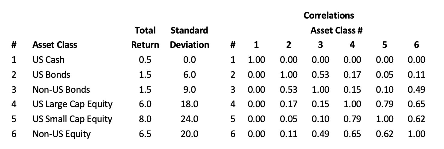
The equity proxy for the options-based product is U.S. large-cap equity, which is the S&P 500. The assumed dividend yield for equities is 2%, which is slightly above the yield on the S&P 500 as of December 31, 2020, which was 1.5%, but is similar to the average dividend yield of the S&P 500 from 2000 to 2020 (1.9%). Dividend yields are an important assumption for the Black-Scholes calculations.
The base implied-volatility assumption for the Black-Scholes model is 25%, which is slightly below the level of the CBOE S&P 500 one-year volatility index as of December 31, 2020 (27.6%), but higher than its longer-term average.2
The volatility (i.e., standard deviation) level for U.S. large-cap stocks is assumed to be 18%, which is below the implied volatility but more consistent with the long-term average. Implied volatility has historically been between 2% and 5% higher than realized volatility, depending on the historical period and respective proxy.
Cash is assumed to be a risk-free asset and used as the base interest rate assumption for the Black-Scholes pricing model.
Four different options-based strategies are considered for the analysis. The first two are floor strategies at 0% or 10%; and the second two are buffer strategies at 10% or 20%. The underlying option prices for each strategy are determined using the Black-Scholes pricing model, which accounts for the implied-volatility smirk noted in part 3 of this series. The caps for the strategies using the base assumptions for the analysis are approximately 1%, 10%, 20%, and 10%, respectively, for informational purposes.
The approaches considered are relatively simple and could easily be recreated by a sophisticated investor or financial advisor with over-the-counter options. The strategies are also consistent with approaches available, such as FIAs (0% floor), RILAs (10% floor, 10% buffer, and 20% buffer), or other products (e.g., buffered ETFs).
While options-based strategies can offer more attractive return distributions than traditional long-only investments, the diversification benefits of options-based strategies vary significantly depending on the underlier. For example, the underlier for the options-based strategies in this piece is the S&P 500. This means the correlation between the options-based strategies and the return of the S&P 500 is relatively high. For example, the correlation between the 10% floor and the S&P 500 price return is approximately 0.85 when the underlier is negative and 0.70 when the underlier is positive; the correlation between the 20% buffer and the S&P 500 price return is approximately 0.60 when the underlier is negative and 0.85 when the underlier is positive. However, these correlations vary significantly depending on the assumptions (e.g., the options budget). Therefore, the positive attributes of the reshaped return distribution are at least partially offset by the higher relative correlation to risky compared to safe assets (e.g., fixed income).
One approach to improve the diversification benefits of the options-based strategies is to select an underlier with a lower market correlation, especially if that investment is not used in a more traditional portfolio. This is something I may explore next.
Optimization results
The exhibits below include the aggregate respective weights to the primary asset classes for the four strategies considered across the risk-aversion levels.
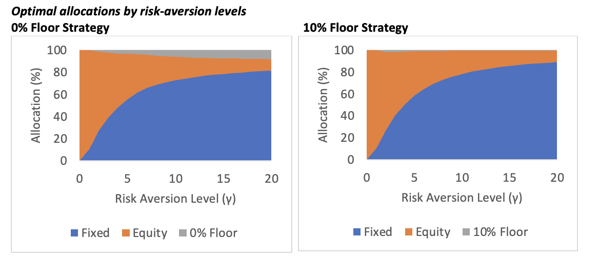
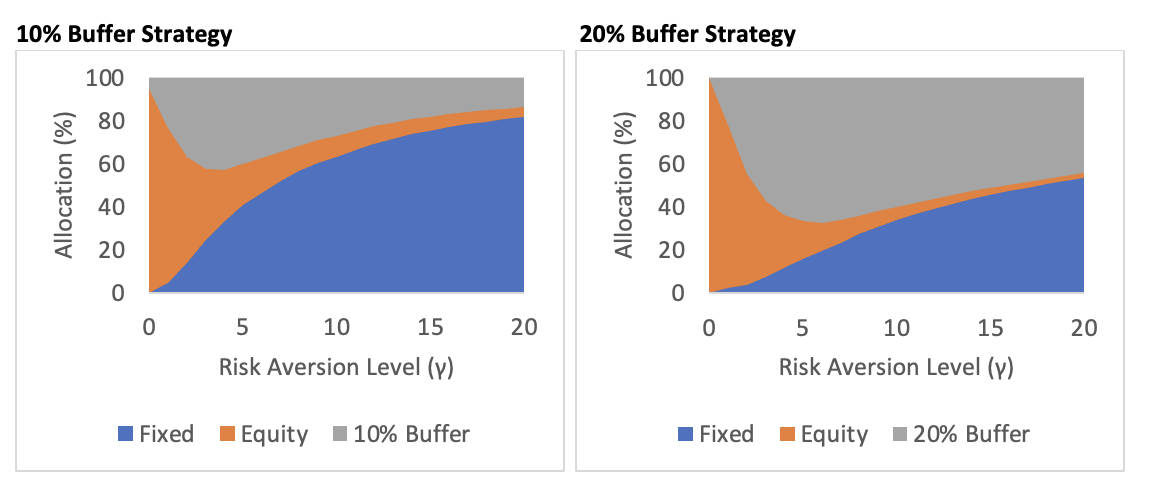
The allocations to the options-based strategies varied significantly by structure. The buffer approaches had higher allocations than the floor approaches. The 20% buffer strategy had the highest allocations, exceeding 60% for moderate risk-aversion levels (e.g., risk aversion levels of approximately 6, which would correspond to an equity allocation of 35% if the options-based strategies are excluded), although the allocations were still significant even for relatively risk-averse investors who would typically invest almost entirely in cash. The 10% floor strategy had the lowest allocations, the greatest being 2% for risk-aversion levels of 3, which correspond to an equity allocation of approximately 60% if the options-based strategies are excluded).
The buffer strategies “soaked up” some of the equity allocation for the moderately risk-averse investors. The buffer strategies are risky, but less risky than directly owning the underlier (the S&P 500), given the buffer. A key reason the buffer strategies received significantly higher allocations than the floor strategies is the cost structure implied within the options pricing model, which I explore more fully in the next section.
Next, for robustness purposes, I varied some of the key assumptions to determine what, if any, effect it would have on the results. I considered four key variables: the price return of equities (-4% change, no change, and +4% change), the assumed return on cash (no change, +1%, and +2%, which affects the investor’s return, not the options budget), the options budget (no change, +1%, and +2%), and implied volatility (no change and -5%, which would be 20%).
Equity returns are varied to reflect uncertainty, especially given high market valuations. The options budget is varied to reflect that issuers of these products have use rates that exceed government bonds to generate the options budget (this was discussed in part 2); however, there may also be additional fees that reduce the realized increase (and liquidity restrictions). The higher returns on cash are included to replicate the higher return available through financial products, such as fixed-rate annuities (also referred to as multi-year guaranteed annuities, or MYGAs) that have similar illiquidity features such as FIAs and RILAs that require dedicating money to a given strategy for some fixed period, such as five years. Implied volatility is adjusted to determine its impact on options pricing.
The allocations to the respective products are included below using the base assumed implied volatility level (25%) for four risk aversion levels: 2, 4, 8, and 20, which roughly correspond to equity allocation targets of approximately 70%, 50%, 30%, and 10%.
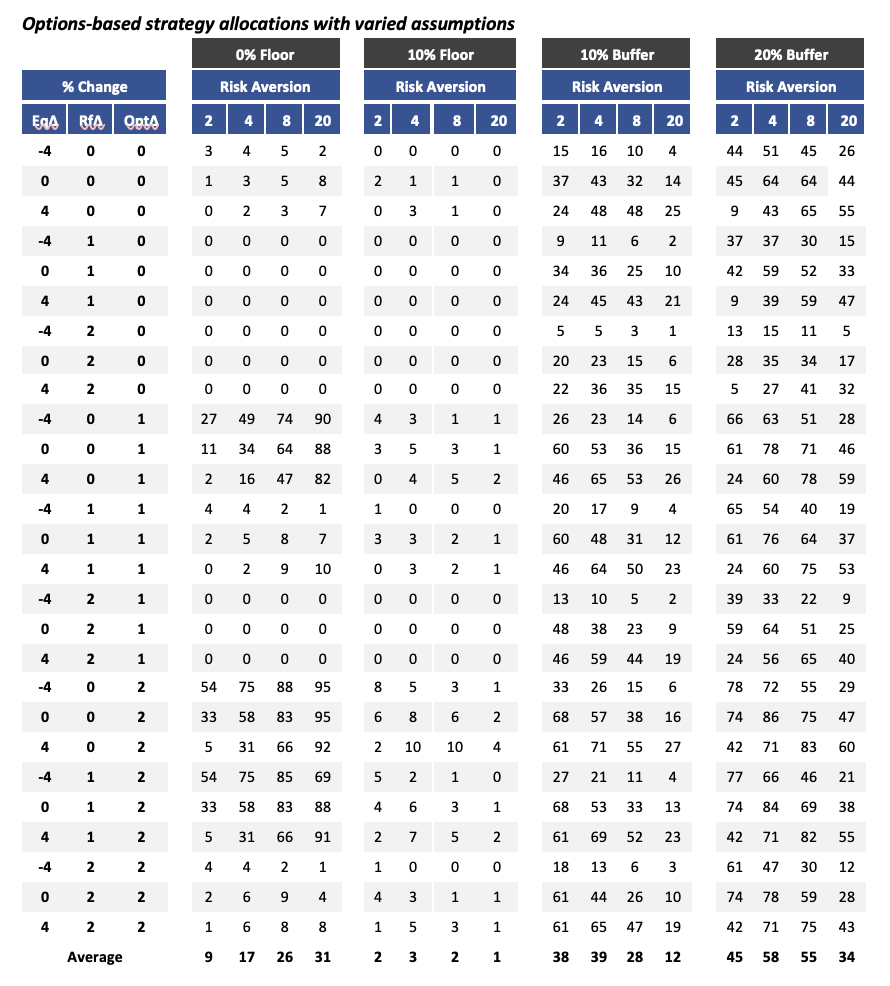
The allocations to buffer and floor strategies increase as the options budget increases and with lower assumed returns on cash. The impact of the changes in the price return of equities was inconsequential based on the changes in other assumptions and the risk aversion level, but is generally higher with higher equity returns.
The most notable change in allocations was for the 0% floor strategy, which is similar to a FIA; it increased considerably when the options budget was increased, even by 1%, holding the other assumptions constant.
The 10% floor strategy allocations did not generally change, even when the options budget was increased. This suggests the 10% floor strategy is dominated by some combination of cash and the other risky assets available, at least given the key assumptions of this analysis.
Conclusions
Options-based strategies can be attractive for investors, but the optimal allocations vary significantly based on the key assumptions. Buffer strategies appear to hold the most promise, provided investors are comfortable with the tail-risk exposure even if accompanied by higher caps (e.g., compared to floors). Floors can definitely still make sense, though, especially those with no downside risk (e.g., FIAs).
In future research I plan on exploring topics like approximating the effective risk of various floor and buffer strategies, as well the benefit of using an underlier that would not typically be in the regular opportunity set (e.g., the S&P 500) since it reduces the potential diversification benefit of the approaches.
David Blanchett is head of retirement research for Morningstar Investment Management LLC. Views expressed are his own and do not necessarily reflect the views of Morningstar Investment Management LLC. This blog is provided for informational purposes only and should not be construed by any person as a solicitation to effect or attempt to effect transactions in securities or the rendering of investment advice.
1 Technically, if the risk aversion level is 1 it is assumed to be 1.01 so the exponent is not 0.
2 https://www.CBOE.com/us/indices/dashboard/VIX1Y/#vix1y-performance
Membership required
Membership is now required to use this feature. To learn more:
View Membership BenefitsSponsored Content
Upcoming Virtual Events View All


