Advisor Perspectives welcomes guest contributions. The views presented here do not necessarily represent those of Advisor Perspectives.
This is the third of my four-part empirical research into the fallacy of the random walk view of investment reward and risk. Part 1 and Part 2 discussed the random walk's failure in portraying asset returns. A random walk depicts risk as volatility.
This article explains why this view is problematic. Risk and volatility are different conceptually. The bell-curve understates actual risks by huge amounts. For asset returns that are not bell-shaped, volatility has no meaning. Finally, volatility is akin to noise, which alleviates instead of elevating risk.
In part 4, I will define investment reward and risk mathematically. I will demonstrate how this probability-based framework enables investors to beat the S&P 500 total-return with less risk.
Risk and volatility are conceptually different
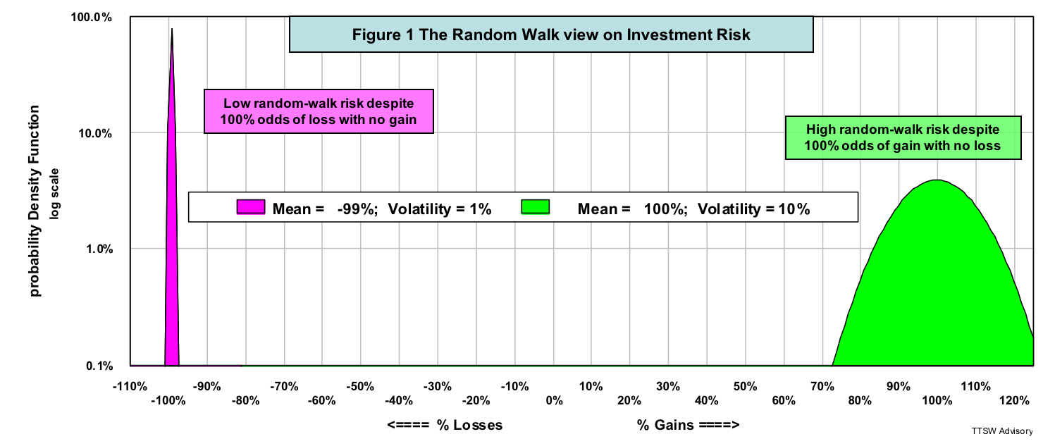
Volatility is a measure of uncertainty in a bell-shaped distribution. The academics define risk as uncertainty primarily for mathematical convenience. Glyn Holton argued that if risk were akin to uncertainty, then a man jumping out of an airplane without a parachute would face no risk because his death was 100% certain. Figure 1 illustrates Holton's argument in an investment context. The green dune at the bottom right is an investment with an expected value of 100% and a volatility of 10%. The pink spike on the left is another investment with an expected value of -99% and a volatility of 1%.

From a risk perspective, modern finance favors the pink investment that offers a 10 times lower volatility than the green one. Investors, however, would intuitively avoid the pink investment because they see the 100% odds of a total loss with no chance of any gain. The academics view the green investment as more risky because it is 10-times more volatile than the pink one. Investors would jump on the green one because they see near 100% odds of doubling their money with zero chance of any loss.
Figure 1 illustrates the conceptual flaw in the random walk notion of risk. Outcome uncertainty is not necessarily risk. Risk is an unacceptable loss.
Random walk grossly underestimates risk
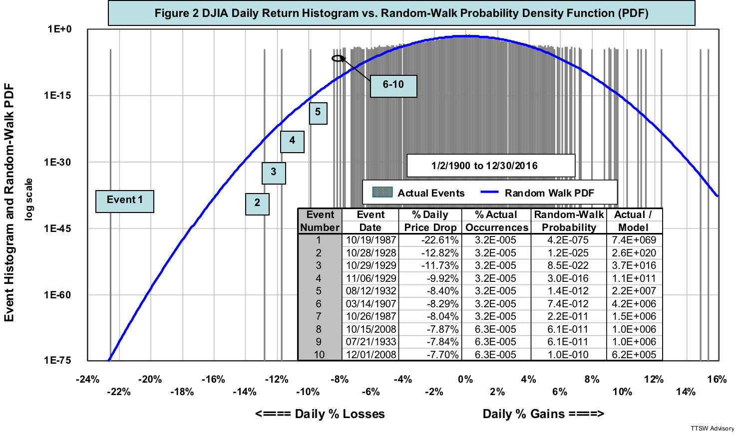
Benoit Mandelbrot points out in The Misbehavior of Markets that Gaussian statistics (random walks) that are behind modern finance grossly underestimate the probabilities of many stock market crashes. To find out how way-off the random walk predictions are, I computed the probability density function (PDF) of the daily returns of the Dow Jones Industrial Average (DJIA) using a measured mean of 0.03% and a standard deviation of 1.24% (from Figure 7 in Part 1). The dark blue curve in figure 2 is the random walk PDF showing the model's predictions of the DJIA's one-day price changes in 116 years (data sources: MetaStock and Yahoo Finance).
The inset table in figure 2 lists 10 of the worst one-day drops in 116 years. On October 19, 1987, for instance, the DJIA dropped -22.61%, a decline that the random walk PDF predicted to have a probability of only 4.2E-075 (the fifth column in the table). To grasp the magnitude of this miss, I use the age of our universe (roughly 14 billion years or 1.4E+010) as the unit of measure. A 4.2E-075 probability means that the Black Monday crash should have occurred only once in a billion billion billion billion billion billion billion times the age of our universe – one followed by 64 zeros. The probability is practically zero.
In reality, the actual frequency of occurrence of each of the seven worst events including Black Monday is 3.2E-005 or 0.0032% (one event out of 31,793 trading days from 1/2/1900 to 12/30/2016). A probability of 0.0032% may be small, but the impact of a one-day crash of -23% was enormous. To make things worse, those bad days tended to cluster – five times from 1928 to 1933, twice in 1987 and twice in 2008.
Volatility is a meaningless metric except for bell-shaped distributions
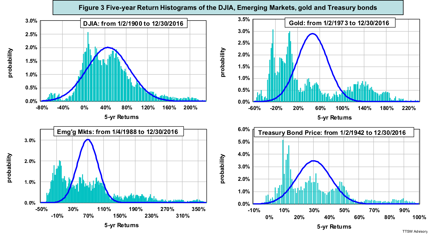
Even if we disregard the conceptual flaw and ignore the huge errors of viewing risk as volatility, we still face with an operational issue. Volatility only works as a statistical yardstick in an ideal bell curve. In the real world, most asset histograms are not bell-shaped. Figure 3 (taken from Part 1 and Part 2) shows five-year return histograms of four widely diverse asset classes (light blue bars). None of them resembles the corresponding random walk PDFs (dark blue curves). The notions of mean and variance are not workable in these wild histograms.
Modern finance doctrines such as Markowitz's portfolio selection, Sharpe's beta and Black-Scholes' risk neutrality view the world through a random walk lens describing everything in terms of means and variances. Figure 3 shows that in the real world, there is no central mean or recognizable variance. It comes as no surprise that many investment strategies based on these doctrines failed to protect investors against risk during financial market meltdowns.
Modern finance confuses risk with noise
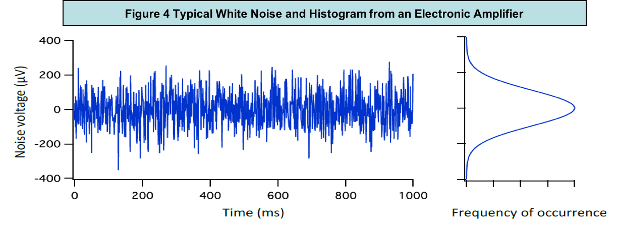
The left chart in figure 4 is a typical noise output of an electronic amplifier measured with an oscilloscope. The right chart is the corresponding histogram. Noise in an amplifier shares the same mathematical root as volatility in asset prices.
I constructed a simulated price series using the random walk pricing model outlined in the Appendix. Figure 5 is a simulated DJIA index computed with Equation (A1) along with its daily returns computed with equation (A2). The band labeled "Random-Walk Daily % Change" in Figure 5 looks very similar to the amplifier noise band in Figure 4 because both are Gaussian. What the academics define as investment risk is what electrical engineers call white noise.
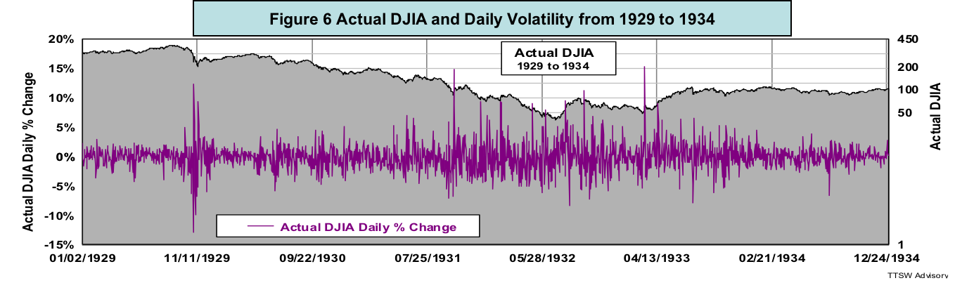
Then what is risk?
Figure 6 shows the actual DJIA and its daily percent changes from 1929 to 1934. The white noise band labeled "Random-Walk Daily % Change" in Figure 5 is uniform and well behaved within ± 1.5%. The band labeled "Actual DJIA Daily % Change" in Figure 6 is erratic and thorny with sharp spikes extended beyond ± 10%. The uniform band in Figure 5 is noise. The negative spikes in Figure 6 are risks. Noise is akin to volatility – uncertainty in the outcomes. Risk is associated with the harmful impact from a negative outcome.
Finally, I use two NASA incidences to illustrate the key difference between noise and risk. The Hubble Space Telescope had a defective mirror that caused spherical aberration that distorted its signals. As a result, Hubble's signals were noisy. The Space Shuttle Challenger broke apart shortly after launch due to improper O-rings. As a result, seven astronauts lost their lives. The Hubble fiasco was a noise issue leading to fuzzy images. The Challenger disaster was a risk matter resulting in deaths. Noise and risk are materially different.
Concluding remarks
The academics envision investors strolling down Wall Street with random movements, but at a smooth and orderly pace. Such tidy bell-shaped randomness is volatility. In reality, investors do not walk in small steps; they jog, run, jump and even take giant leaps, and deep dives, creating turbulence and chaos in the financial markets. Such violent footprints are risks.
Volatility measures fluctuations and risk signifies dangers. They are not synonymous as modern finance claims. Fischer Black in his 1986 article entitled Noise argued that volatility was a risk-reducing agent. When there is diversity (noise) in market views, prices will fluctuate, giving rise to volatility. Volatility is the mechanism through which buyers and sellers carry out normal price discoveries. Noise facilitates transactions and volatility alleviates risk in the financial markets. In contrast, a market that has only one prevailing belief is noise-free. Prices no longer fluctuate but charge in the direction of the dominant view. When the bears coalesce and become the majority, liquidity will dry up, panic selling will set in and risk will surge.
By defining risk as volatility, the random walk theorists create a paradox. When price fluctuations are less than ± one standard deviation from the mean, the bell curve has some resemblance to the real world. In the central region of the bell curve, however, volatility is not risk but a risk stabilizer. At the tail ends of the bell curve, where real risks reside, volatility is a meaningless metric because Gaussian statistics no longer work.
In the next and final article, I will define both investment reward and risk using a framework different from the random walk paradigm. Like the random walk, my new framework has firm probability underpinnings. Unlike the random walk, my new formulas are applicable to all probability distributions regardless of their shapes and forms. More importantly, the new model yields new insights on how to increase the odds of beating the S&P500 total return with less risk – a direct challenge to Efficient Market Hypothesis.
Theodore Wong graduated from MIT with a BSEE and MSEE degree and earned an MBA degree from Temple University. He served as general manager in several Fortune-500 companies that produced infrared sensors for satellite and military applications. After selling the hi-tech company that he started with a private equity firm, he launched TTSW Advisory, a consulting firm offering clients investment research services. For almost four decades, Ted has developed a true passion for studying the financial markets. He applies engineering design principles and statistical tools to achieve absolute investment returns by actively managing risk in both up and down markets. He can be reached at mailto:[email protected].
Appendix: The Random-walk Pricing Model
The random walk pricing model relates the price at time T + ΔT (Price T + ΔT) to the price at time T (Price T) with the following formula:
Price T + ΔT = Price T x [1 + Mean ± Volatility]. (A1)
Dividing both sides of Equation (A1) by Price T and rearranging terms, one obtains:
(Price T + ΔT / Price T) - 1 = Mean ± Volatility. (A2)
Equation (A1) is a simulated random walk price series. Equation (A2) is the return (rate of change) on that price series within a time increment of ΔT.
In the above two equations,
Mean = Expected Value (Cumulative Probability Weighted Return); and (A3)
Volatility = N x Standard Deviation, (A4)
The sign and the amplitude of N can be simulated using a Gaussian noise generator with a bell-shaped probability distribution.
To create a daily (ΔT = 1 day) DJIA time series, I use a mean of 0.03% and a standard deviation of 1.24%, the same parameters obtained from Figure 7 in Part 1, which were used to compute the DJIA daily return PDF in figure 2.
Read more articles by Theodore Wong
 Then what is risk?