Advisor Perspectives welcomes guest contributions. The views presented here do not necessarily represent those of Advisor Perspectives.
In my prior articles (here and here), I evaluated a series of methods for obtaining retirement income from savings, leading to two strategies that perform best over a broad range of market conditions and “tilts[1].” The first strategy is a constant-rate method with “tilt” from slightly negative to strongly positive. The second strategy, the mortgage method, takes advantage of finite lifetime to increase income and was found to outperform mortality based methods that appear to be similar but are not. This article examines how the best performing strategies can be combined with annuities, pensions, Social Security and different tilts to allow clients to best choose between capital preservation and income stability.
My simulation assumptions were identical to the prior companion article except as noted: returns consistent with Vanguard 10-year predictions, an asset allocation of 80% world stock, 20% bonds was assumed (annual real return 5.3%, standard deviation 0.11) and an annuity payout for a 65-year-old female of 4.5% (Income Solutions Quote, CPI adjusted). Social Security is assumed to provide $25,000 of income.
The graphs are shown with 0%, 25%, 50% and 75% of the initial capital converted to a single-premium immediate annuity (SPIA) at the start of retirement (female age 65). Those correspond approximately to 38%, 55%, 70% and 85% (respectively) of the anticipated income coming from the guaranteed income portion (Social Security + pension + SPIA).
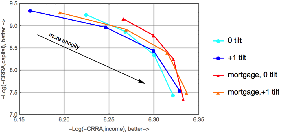
I used a constant relative risk aversion (CRRA) utility function with a risk-aversion factor of four and simulated over two million person-years (for each dot/triangle marker in the graphs that follow). The utility function results were dominated by periods when either capital or income became low for an extended period (Figure 1). Two functions were calculated: one for the annual income and one for the capital balance. The income for the utility function was adjusted at a rate of 2%/year to reflect the observed pattern of lower spending with age. The arrow shows how to align the four markers in each line with the fraction of initial capital placed into the SPIA. All the selected methods perform well and have regions where they are superior. By selecting method, tilt and degree of annuity, the client can be placed anywhere along the top surface of the figure (i.e., the efficient frontier). Relatively high tilts along with zero tilts were simulated to illustrate the range available with intermediate tilts. The graphs steepen at higher levels of annuitization, suggesting that the amount of annuities should range from 25-50% of initial capital (guaranteed income 50-75%) in order to balance income and capital risk. High positive tilts should be applied with a greater fraction of annuitization.
Figure 1. CRRA utility function measures risk of low capital or low income during any time period of any realization.

For example, in the above graph, the horizontal axis represents the utility function score for annual income and the vertical axis represents the utility function score for annual capital balance. The dark blue line represents a constant-rate strategy with +1 tilt. The blue dots from left to right along this line represent 0%, 25%, 50% and 75% of initial capital placed into the SPIA. As the proportion of SPIA increases, the capital utility decreases (i.e., less capital remains) while income utility increases (i.e., SPIA stabilizes the income). Moving from left to right on the figure, each additional aliquot of SPIA results in a greater loss in capital utility with a correspondingly smaller increase in income utility.
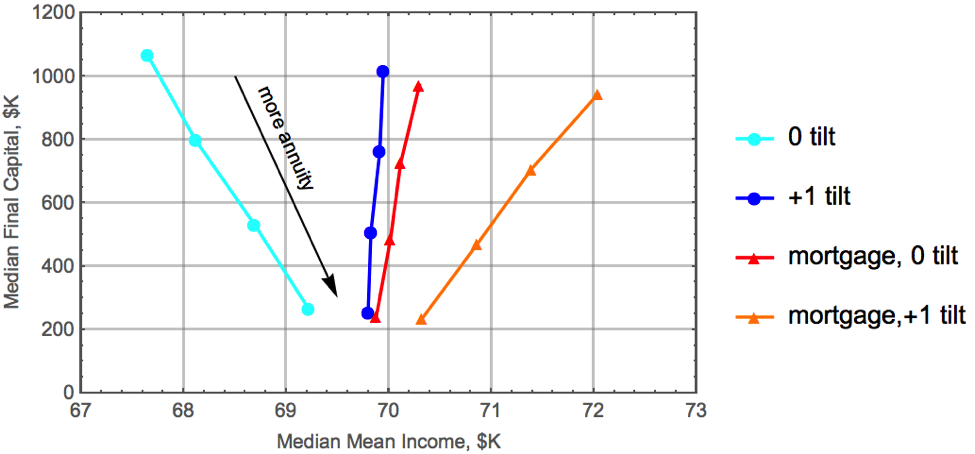
Median/anticipated results (Figure 2) illustrate the tradeoff between final capital at death (bequest) and anticipated income. Death occurs at any age past 65 based on mortality tables (single female). All methods work well. Depending on the method chosen, annuities either increase or decrease the income, but the range is small. The tilted options produce higher incomes. Under the same conditions, the 4% rule would have provided $65,000 income.
Figure 2. Median results with 0, 25, 50, or 75% of initial capital spent on SPIA on date of retirement (38, 55, 70, and 85 percent of anticipated income coming from guaranteed sources (social security + pension + annuity).
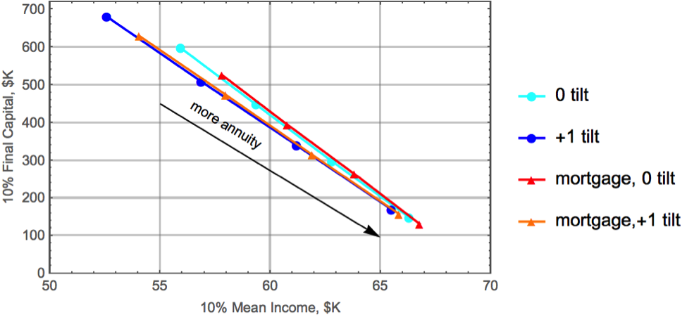
Given the high volatility of the assumed 80/20 asset allocation, returns over a finite period can be much higher or lower than anticipated. The bottom 10th percentile results are shown in Figure 3. The positively tilted methods are designed to preserve capital when markets are poor, and that effect is clear in the results. All the incomes are lower, especially for the no or low annuity options.
The slope of the line that all the methods tend along is $2,500 annual income/ $100,000 capital at death. Annuities have payout rates greater than this slope. The tilted methods in the upper left have preserved sufficient capital for annuities to be purchased later in life if more income were desired. The delayed purchase would be cost effective even subsequent to relatively poor (mostly negative in this case) market returns.
Figure 3. Bottom 10th percentile of simulations representing unfavorable market outcomes.
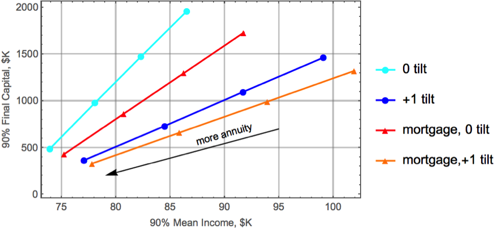
Figure 4 gives favorable (90th percentile) market results. Annuity purchases (insurance) lower income when market returns are high. All the methods automatically shift toward higher income.
Figure 4. Superior market returns provide higher income than annuities.
None of the recommended methods ever go broke, and the remaining capital never cascades irreversibly toward zero. There is no sequence-of-returns risk and very little longevity risk. The tradeoff is income stability. Income varies each year, and if returns are poor, income will suffer unless stabilized with annuities.
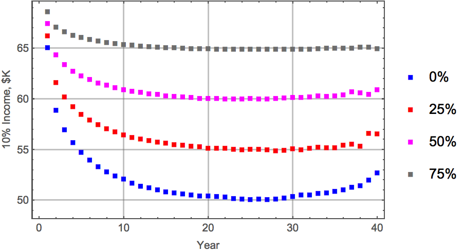
Figure 5 illustrates the mortgage method with a slight positive tilt (+1/3) at the lower 10th percentile of annual income. The percentage labels (right vertical axis) are the fraction of initial capital annuitized on the day of retirement. The traces are not time histories of individual clients, but rather a slice of the income distribution of the survivors. The overall probability of each point is 10% times the probability that a 65-year-old female lives to the corresponding age. Typically, an individual client would only slide into the bottom income percentiles on the figure for a year or two before market and income recovered. The annuities supply a robust floor on the annual income. Notice that the lower 10th percentile income stabilizes after about 15 years of retirement, even with continued poor market returns. The +1/3 tilt has automatically re-calibrated the system to be stable at the lower 10th percentile of market returns, thereby eliminating longevity risk for this low return scenario.
Figure 5. Mortgage method, +1/3 tilt showing lower 10% of income from surviving clients each year of retirement (age = 64+ year).
How to apply the methods
The two classes of methods illustrated are constant rate and mortgage, each with and without tilt. This spreadsheet illustrates application of both classes. The method, tilt and degree of guaranteed income (annuity + pension + social security) are chosen by examining Figures 1-5 above. The estimated income from each method assuming an initial $1,000,000 of capital can be obtained by subtracting Social Security ($25,000) from the figures. All methods were set to provide $40,000 of income in the first year.
Observations:
- The methods all respond dynamically to market conditions and thus do not suffer sequence-of-returns risk and minimize longevity risk. The rapid response of income to market performance has many benefits for increased financial security and overall income, but does mean income will vary from year to year. Annuities provide a critical floor for the annual income (Figure 5).
- An advantage of the mortgage method with or without tilt is that it automatically increases income if the client retires at an older age (and decreases it if the client retires at a younger age). There is no need to rerun the simulations for substantially different retirement ages relative to the age 65 assumed here.
- When combined with guaranteed income, the positive tilts provide a very robust combination of high stable income and capital security over a broad range of market conditions. They combine the statistical advantages of annuities – safe return of capital and mortality credits– with the statistical advantages of positive tilts – providing income that adaptively matches market returns while preserving capital.
- I performed identical simulations with the Vanguard 60/40 stock/bond return predictions, which gave universally inferior results to the 80/20 portfolio results. As Wade Pfau has written, bonds are inferior to annuities (SPIAs) in retirement portfolios; a higher portion of annuities always beats a higher portion of bonds. I did not perform a 100% stock simulation because every client needs an emergency fund, and the emergency fund should not be in stocks.
- I also performed identical simulations at an annual real return of 3.3% and a standard deviation of 0.11. All the methods worked well. Incomes were lower and annuities more favorable.
- If the client has health issues and is unlikely to live to old age, the mortgage method with a shorter but still conservative maximum lifetime should be used.
- If the client purchases a deferred-income annuity (DIA) to provide certain income late in life, then the mortgage method can be set to terminate a few years after the annuity begins.
- The mortgage method, with more conservative investments, can be used with a portion of the initial capital to delay social security until age 70. In this case the termination date is age 70.
- If the client has a strong bequest motivation, a high tilt is appropriate.
- High tilts, with their capital preservation bias, work well with annuity purchases sequenced over time.
- If the client refuses annuities and doesn’t have high Social Security and/or pension to compensate, the tilt should be small or even negative (-0.25 to +0.25) to avoid high income variability. Bonds would also have to be added to the portfolio in proportion to the annuities in the figures.
- There are many ways to provide a positive tilt, including an advisor who steps in to modify withdrawals when assets and income become misaligned. Tilt doesn’t have to be applied with a formula.
- If equity markets’ mean revert, the positive tilts will perform better than simulated. Mean reversion is not included in the Monte-Carlo and is not the source of the illustrated benefits from tilting.
John Walton is an engineering professor at the University of Texas at El Paso, where he has taught for 24 years. He has a Ph.D. in Chemical Engineering. His interest in financial planning came from considering options for his coming retirement.
[1] The tilt is a factor that adjusts the withdrawal rate relative to the remaining balance. If the withdrawal rate is 4%, then a positive tilt will decrease the withdrawal rate below 4% if the balance was below the target level and increase the withdrawal rate above 4% if the balance was above the target level. The degree of adjustment depends on the magnitude of the tilt.
Read more articles by John Walton