A Comparison of Variable Spending Strategies
Membership required
Membership is now required to use this feature. To learn more:
View Membership Benefits This is part two of a two-part series. You can read part one here.
In part one of this series, I established a framework for evaluating variable spending strategies in the context of retirement planning. My framework used a “PAY” rule that integrated the probability (P) that the remaining portfolio balance falls below a threshold amount (A) of (in inflation-adjusted terms) by year (Y) of retirement (Probability, Amount, Year). I evaluated a constant real spending strategy (motivated by William Bengen’s original research on the 4% rule) using this framework and illustrated a number of drawbacks in this approach.
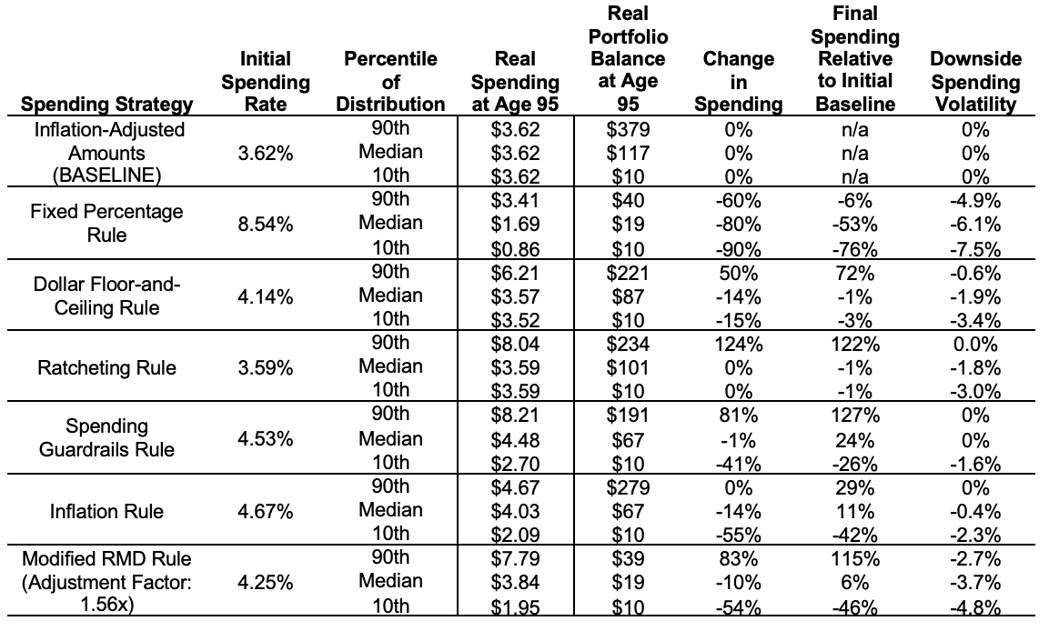
Let’s analyze the remaining strategies using this framework. Those strategies were in exhibit 1 in part one of this series, reproduced here:
Fixed-percentage rule
On the spectrum of spending strategies, the fixed-percentage rule shown second is the opposite of constant inflation-adjusted spending. It calls for retirees to spend a constant percentage of the remaining portfolio balance in each year of retirement. Occasionally the popular press will mistakenly define the 4% rule this way (a 4% fixed percentage strategy calls for withdrawing 4% of the remaining account balance each year), but the accepted definition of the 4% rule is the constant inflation-adjusted spending strategy described in part one. To be clear, with constant inflation-adjusted spending, the nominal withdrawal rate will change throughout retirement as the portfolio value and inflation rate change. The withdrawal rate adjusts, while spending stays the same. But with fixed percentages, the withdrawal rate stays the same, while spending adjusts.
An advantage of the fixed-percentage strategy is that, since it always spends a percentage of what remains, it never depletes the portfolio. Of course, spending could fall to uncomfortably low levels, but the concept of portfolio failure rates is inapplicable here. In addition, spending increases when market returns outpace the spending rate and the portfolio grows. As well, this strategy eliminates sequence-of-return risk, as the late and esteemed Dirk Cotton first pointed out in 2013 at his Retirement Café blog. The fixed-percentage approach provides a clear mechanism for reducing spending after a portfolio decline. As with investing a lump sum of assets, the specific order of returns makes no difference to the final outcomes realized with this strategy. As such, we can expect the sustainable spending rate to be higher than with constant inflation-adjusted withdrawals. With our PAY rule calibration, this strategy allows initial spending to begin at 8.54%, which is more than double the initial spending with the baseline strategy.
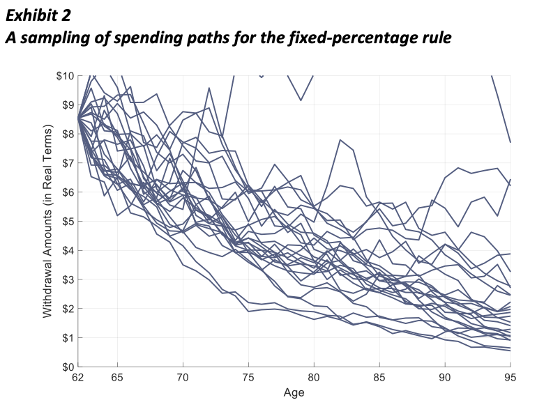
As for disadvantages, volatile investments result in extremely variable spending, making it difficult for retirees to plan a budget. Though spending begins at the greatest level, this strategy experiences the largest spending reductions and downside spending volatility. It is a clear example of the trade-off between allowing for a higher initial spending rate and less spending for later in retirement. For a fixed retirement budget, managing retirement with this rule could be a challenge. Those considering this rule should be thinking in terms of applying it to discretionary expenses that allow more flexibility for spending reductions that will not derail a retiree’s standard of living. This spending strategy also strongly front-loads the spending for those seeking to maximize lifestyle in their early retirement years, and it efficiently spends down assets to leave the smallest legacies at the end of retirement. Exhibit 2 illustrates the path of retirement spending for a random sampling of spending paths with this rule.
With these advantages and limitations in mind, recall that the fixed percentage rule is the opposite of constant spending. Most practical approaches to flexible retirement spending seek to balance the tradeoffs between reduced sequence risk and increased spending volatility by only partially linking spending to portfolio performance. Let’s consider some of the main levers used in variable spending strategies that have been proposed by researchers and practitioners.
Floor-and-ceiling withdrawals
For example, Bengen has described floor-and-ceiling withdrawals as one such spending compromise. This method begins by applying the fixed percentage rule, which allows greater spending when markets do well and forces spending reductions when markets do poorly. Bengen added hard-dollar ceilings and floors on spending. Spending is not allowed to fluctuate outside of a specified range. The fixed-percentage rule is applied when spending falls inside the bands and a constant-amount strategy is applied at the ceiling or floor when the fixed-percentage rule would force spending outside of this range. This keeps spending from drifting too far from its initial levels, helping to smooth spending fluctuations to manage sequence risk and allowing for a higher initial spending rate.
The example I used to describe this rule is based on a ceiling that is 50% greater and a floor that is 15% less than the inflation-adjusted value of the initial withdrawal amount. This smooths fluctuations by keeping spending from drifting too far from its initial level. While the hard-dollar floor ensures spending never drops too low, it also restores the possibility of portfolio depletion.
A willingness to reduce spending by up to 15% from the initial level provides a great deal of support for sustaining the investment portfolio in retirement. Placing a ceiling on spending will preserve sustainability by saving more for future “rainy days.”
The initial spending rate is 4.14%. Spending with this strategy is held within the range mentioned. It can reach as high as $6.21 (a 50% increase), which it does at the 90th percentile. On the downside, spending can drop as low as $3.52, which is 15% below the initial retirement date spending level, and 3% less than the amount provided through the baseline strategy.
Downside spending is only slightly less than with the constant inflation-adjusted baseline.
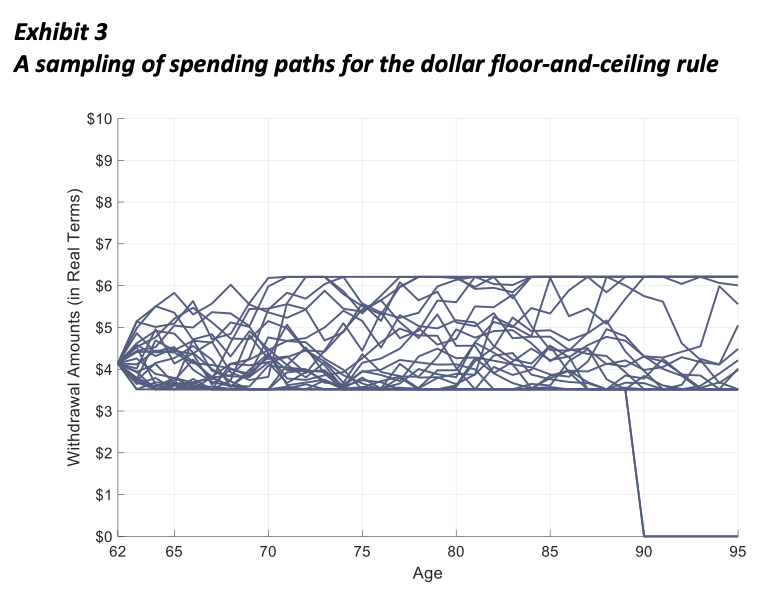
Bengen’s floor-and-ceiling rule allows initial spending to increase while also providing the ability to adjust spending to reduce sequence risk. In this way, even when the floor is reached, spending remains at about the same level as it was with the constant inflation-adjusted baseline strategy. By allowing for higher spending, the floor-and-ceiling strategy does lead to less legacy assets, though the median remaining wealth is the third highest of these rules. This strategy allows for some variability in spending and spending reductions. The average spending reduction at the median is about 2%, while it is 3% at the 10th percentile. Exhibit 3 provides a sampling of spending paths with this rule.
The choice of the ceiling value does not have much impact on sustainable spending. If the portfolio does well enough for spending to grow beyond the ceiling, sequence risk has not manifested. The current withdrawal rate declines. It becomes unlikely that portfolio depletion will be a concern. The important variable is the dollar floor. The lower the floor, the greater the initial withdrawal rate that can be supported.
The ratcheting rule
This observation motivates the next example of a ratcheting rule that is a special case of the floor-and-ceiling rule. It was introduced by Michael Kitces’ in a 2015 blog post, though his rule was dramatically more complicated and did not allow for any subsequent spending decreases. Kitces merely aimed to reveal the superiority of a ratcheting rule versus constant inflation-adjusted spending, and my example shares this aspect of his discussion.
For a simple ratcheting rule, I applied an inflation-adjusted dollar floor at the initial spending rate and no ceiling. This means that the strategy provides constant inflation-adjusted spending when the real value of the portfolio is less than its initial value, but fixed-percentage spending when the real value of the portfolio has increased.
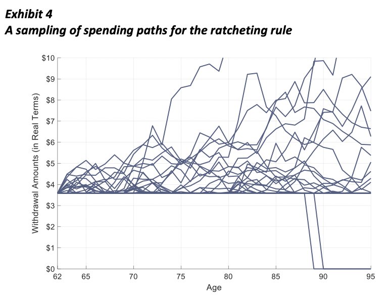
This ratcheting rule supports an initial withdrawal rate of 3.59%, which is slightly less than the baseline strategy. But in the 90th percentile, spending increases by more than 100%, while spending is preserved in inflation-adjusted-terms at the median and 10th percentile. With the ability for spending to increase, there is also downside spending volatility after portfolio declines. This strategy preserves the initial portfolio balance at the median and supports the third highest legacy at the 90th percentile. Exhibit 4 provides a sampling of spending paths with this rule.
The Guyton guardrails
Perhaps the most famous variable spending strategy is the collection of decision rules developed and refined over the years by Jonathan Guyton and William Klinger. Guyton’s initial approach gained traction as he was one of the first to emphasize the possibility of allowing for a higher initial spending rate when flexibility was added to reduce subsequent spending when triggered by a decision rule. This point was included in the title of his original 2004 article (“Decision Rules and Portfolio Management for Retirees: Is the ‘Safe’ Initial Withdrawal Rate Too Safe?”) when he asked whether the “safe” initial withdrawal rate was too safe. Guyton and Klinger developed a series of decision rules that allowed for a greater initial spending rate but provide guardrails around spending to keep the ongoing distribution rate from rising too high as a percentage of remaining assets.
I’ll separate their decision rules into levers for two distinct strategies. First, I will describe simplified versions of their capital preservation and prosperity rules as providing spending guardrails for retirees. Spending guardrails work in the opposite manner of the floor-and-ceiling rule. While the floor-and-ceiling rule defined spending as a fixed percentage with dollar guardrails, these rules use constant amounts with percentage spending guardrails.
Constant inflation-adjusted spending occurs when that spending falls inside the percentage guardrails. The capital preservation rule monitors the current withdrawal rate for this inflation-adjusted spending as a percentage of the remaining portfolio balance. If the portfolio declines and the current withdrawal rate gets pushed too high, the capital preservation rule triggers to prevent spending from rising higher than a set percentage.
The prosperity rule works in the other direction. If the portfolio grows enough for the current withdrawal rate to fall below a defined threshold, then this spending guardrail is triggered to increase spending so that it does not fall below a fixed percentage of what is left.
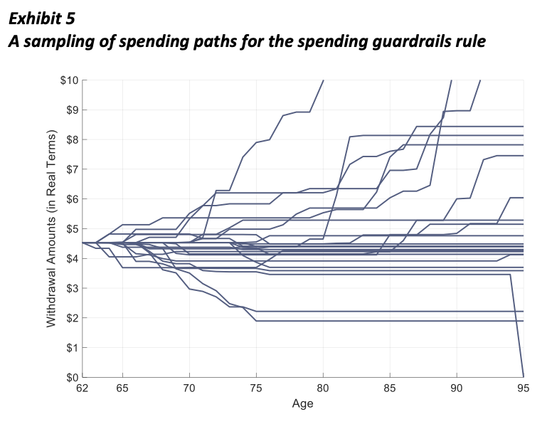
In this example, the supported initial withdrawal rate is 4.53%. The capital preservation rule is that the current withdrawal rate is not allowed to exceed 120% of this value (or 5.44%) for the first 15 years of retirement. When the portfolio declines enough to trigger this decision rule, a fixed percentage rule is applied until either the portfolio recovers so that the inflation-adjusted value of the previous year’s spending is less than this percentage, or the couple reaches age 78. The prosperity rule applied is that spending rate is never allowed to drop more than 20% below its initial level (or 3.62%). When the portfolio grows enough that 3.62% of what is left is more than the inflation-adjusted amount of the previous year’s spending, then the rule switches to a 3.62% fixed percentage distribution. The prosperity rule is used for the entire retirement horizon. The rule does allow for dramatic spending increases at the 90th percentile. For the median, spending stays about the same, which is notably higher than with the baseline strategy. Spending decreases significantly at the 10th percentile.
Exhibit 5 provides a sampling of spending paths with this rule. I include this strategy because it is so well known, but in practical terms I it is not very easy to use it. This is because it is not possible to include the percentage guardrails in the exhibit because they calibrate to the current portfolio value rather than the initial portfolio value. The guardrails evolve based on the remaining portfolio balance in each simulation such that the spending amount triggered by a decision rule depends on the precise value of the remaining portfolio in the year that the guardrail is triggered. The concept of having prosperity-based and capital-preservation-based guardrails was quite important, but other rules I investigated provide a more practical way to implement spending adjustments.
The inflation rule
The other interesting Guyton and Klinger rule, which I separate into a different strategy, is their withdrawal rule, which I will call the inflation rule. It provides a decision rule for determining whether spending adjusts for inflation or remains fixed in nominal terms. The basic premise of his rule is that retirees are willing to forgo an inflation increase but will never want to accept a decrease in their nominal spending. Remember that keeping spending level when there is inflation means that real spending declines.
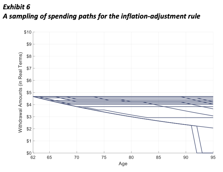
The inflation rule requires a decision rule for when to adjust spending for inflation. I found a simple rule that works just as well as any of the more sophisticated methods I tested. It is to record the nominal balance of the investment portfolio at the start of retirement. Then, in the future, the retirement behavior is based on whether the remaining investment assets are greater than or less than the initial retirement portfolio value at the start of retirement. One compares only the current value of the investment assets with the nominal value at the start of retirement to make the decision. Spending increases for inflation in years when the remaining portfolio balance exceeds its initial nominal value. The inflation adjustment is skipped in any year that the remaining portfolio balance has fallen below its initial value.
This rule supports an initial 4.67% withdrawal rate, which is the second highest with 29% more spending than the baseline rule. By age 95, spending has fallen by 14% at the median and by 55% at the 10th percentile. This strategy supports the second highest legacy at the 90th percentile, since there is no spending increase to take advantage of the good market performance. Exhibit 6 provides a sampling of spending paths with this rule.
Actuarial rules
Finally, another important spending rule uses actuarial methods. Actuarial methods generally call for retirees to recalculate their sustainable spending annually based on the remaining portfolio balance, remaining longevity, and expected portfolio returns. This approach uses an increasing percentage from the remaining portfolio over time to account for the shortening remaining life expectancy as one ages. For various actuarial methods, differences center primarily on appropriate assumptions for market returns and remaining longevity, as well as whether additional smoothing factors should be applied to control how quickly spending adjusts to new circumstances.
A simple form of the actuarial method is to use the Internal Revenue Service’s required minimum distribution (RMD) rules (based on the table III uniform life table) as a general guide for sustainable spending. For the purposes of tax collection, the RMD rules indicate a by-age percentage that must be withdrawn from tax-deferred retirement accounts.
The RMD rule dictates how to spend a percentage of remaining assets, which is calibrated to an updating remaining life expectancy. Its deficiency is that it does not provide a mechanism for users to adjust their portfolio return assumption beyond what government policymakers initially assumed when developing the by-age RMD rates. The RMD tables assume investment returns of 0%, so they do not reflect asset allocation or other capital market assumptions. The standard RMD table also assumes a couple with one spouse 10 years younger than the other. Even though at present RMDs begin at age 73, we can find the rates at younger ages using table II with an age difference assumption. Exhibit 7 shows the withdrawal percentages implied by the RMD rules for ages 62 and older.
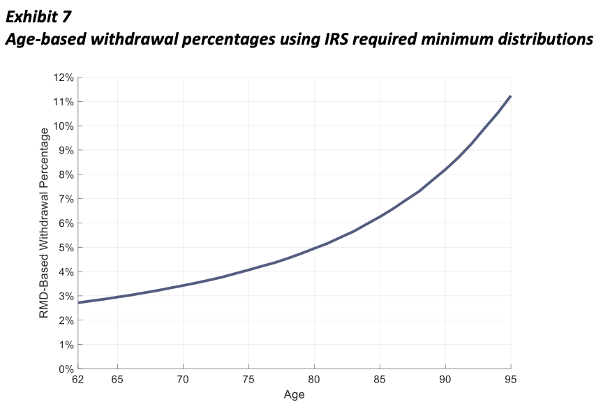
With its conservative returns and assumed age difference, some retirees may decide the RMD strategy provides overly conservative spending rates. For instance, the implied withdrawal rate at age 65 is 2.95%, which may be quite low for a strategy that creates minimal sequence risk, which is caused only by the fact that the percentage is age-based instead of fixed. Another possibility, then, is to increase all the RMD rates by a chosen factor to increase spending.
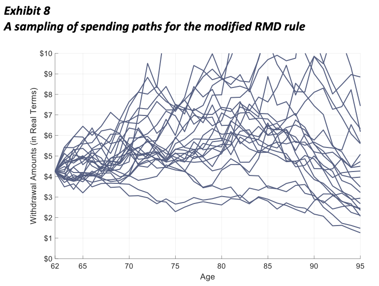
A straightforward application of the RMD rule would not calibrate remaining wealth for the PAY rule. I modified the RMD rates so this calibration may take place. In order to accomplish this, I found the appropriate factor to adjust all RMD percentages so the PAY rule threshold is reached. My modified RMD rule simply multiplies all RMD percentages by 1.56 so that the age 62 RMD percentage of 2.72% is adjusted upward to 4.25%. Subsequent spending rates are based on a percentage of remaining assets required by the rule and multiplied by the same calibration factor. This leads to a strategy with the greatest spend down of wealth. Spending increases dramatically at the 90th percentile, while falling slightly at the median, though it remains greater than the baseline strategy. Large spending reductions can be expected at the 10th percentile, and the downside spending volatility is the second highest after the fixed-percentage strategy. This rule behaves similarly to the fixed-percentage rule, except that it smooths spending over time by starting with a smaller initial percentage but then increasing it. Exhibit 8 provides a sampling of spending paths for this rule.
Bottom line
Any of these variable spending strategies will reduce sequence risk in retirement and allow for greater initial spending rates, potentially greater average spending amounts, and a generally more efficient spenddown of assets than the baseline constant inflation-adjusted spending rule. Incorporating a strategy for flexible retirement spending, at least for discretionary expenses, is an important part of building a comprehensive retirement income plan.
Wade D. Pfau, PhD, CFA, RICP® is a co-founder of the Retirement Income Style Awareness tool, the founder of Retirement Researcher, and a co-host of the Retire with Style podcast. He also serves as a principal and the director of retirement research for McLean Asset Management. He also serves as a Research Fellow with the Alliance for Lifetime Income and Retirement Income Institute. He is a professor of practice at the American College of Financial Services and past director of the Retirement Income Certified Professional® (RICP®) designation program. Wade’s latest book is Retirement Planning Guidebook: Navigating the Important Decisions for Retirement Success.
Membership required
Membership is now required to use this feature. To learn more:
View Membership BenefitsSponsored Content
Upcoming Virtual Events View All


