Historical Returns Distort the Analysis of Annuities

Bond yields driving upside

Bond yields are an important driver for the returns for a variety of investments. Most simply, the yield on a bond sets the expected return for a bond investor, especially one who purchases a government bond (assuming it is risk-free) and plans on holding the bond to maturity.

Bond yields also play an important role in the expected return of other financial products, such as annuities. For example, for accumulation-focused annuities, such as FIAs, which have been available since the mid-1990s, as well as the growing category of “buffer” and “floor” annuity strategies, such as RILAs, index-variable annuities (IVAs), and structured annuities, bond yields help determine the upside of the product (i.e., the cap) since they are a key input to the options budget.

This effect is most easily described with a FIA. If an insurance company can buy bonds yielding 2%, ignoring other expenses, it can use that 2% yield to purchase options that generate the upside potential. The higher the yield, the more money that is available to purchase options to generate the product’s upside potential (i.e., the cap).

Options prices

To better understand how options prices have responded to changes in bond yields, I obtained data on historical options prices from DeltaNetural.com on the SPX (i.e., the S&P 500). Since options with a precise one-year expiration are not generally available, I used interpolation and ran a series of regressions to estimate the rolling cost of one-year options.

My analysis attempts to estimate the caps for a FIA with a one-year annual point-to-point crediting approach with a 100% participation rate. Given the options prices, the options budget is set based on historical AAA bond yields and no expenses are assumed. The yield on AAA bonds was 2.55% in August 2021.

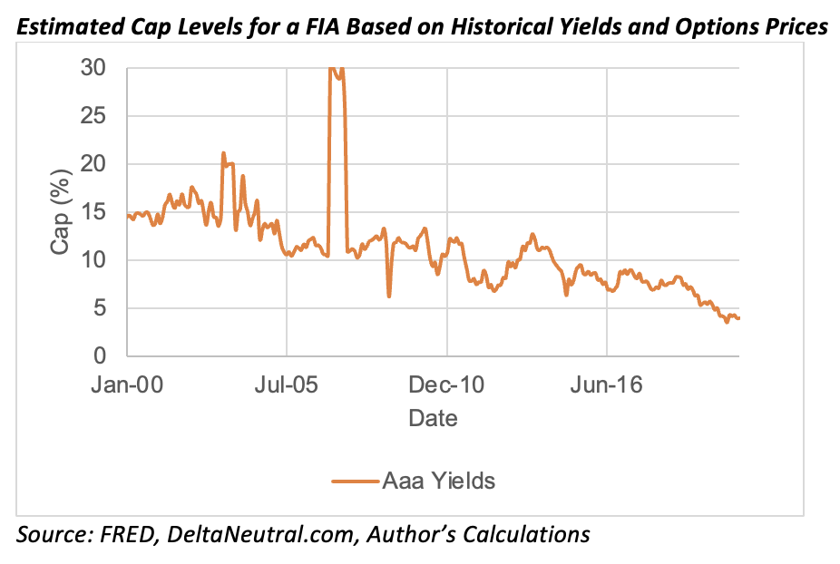
As bond yields have declined over the past two decades, the estimated caps for a FIA have decreased significantly. This analysis suggests caps today should be approximately 5%, which is currently consistent with actual caps on FIAs.

While there are a variety of factors that drive options prices, bond yields are a key component. In the next exhibit, I demonstrate the relationship between AAA yields and estimated caps.

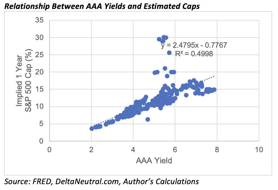
Not surprisingly, caps have historically been higher when bond yields have been higher. This is important especially when thinking about how yields have evolved over time and the extent to which you can use caps at a given point-in-time for a longer-term analysis.

For example, FIAs were introduced in the mid-1990s when yields were around 8%. The estimated cap when yields are 8% would be approximately 15% based on the previous exhibit. In contrast, when AAA yields are around 2.5% (closer to where they are today), caps are closer to 5%, which is significantly lower.

Caps evolve with interest rates over time; therefore, a cap based on a current rate environment should not be “back tested” in previous yield environments where the yield was significantly different.

Here is a general rule of thumb regarding AAA yields and cap rates: For one-year annual point-to-point FIAs on the S&P 500 with 100% participation rates, cap rates should be approximately 2.5 times the underlying yield of AAA bonds (the slope coefficient in the previous regression). This effect was noted by David Lau, founder and CEO of DPL Financial Partners, when reviewing a draft of this piece. Given a median historical yield on AAA bonds from 1919 to 2021 of approximately 5%, would suggest an analysis using pure historical returns should assume a cap closer to 12.5%, versus the lower caps available today (which would be closer to 5%).

Going even further back

This need to view caps as a function of then-prevailing interest rates becomes more obvious if we extend our analysis to before the year 2000 and use the Black-Scholes options pricing model to estimate how caps would have evolved since 1919 (when AAA yields were first available).

The implied volatility assumption for the at-the-money options in the Black-Scholes options pricing model is assumed to be 25% for the entire historical period, which is consistent with the average historical implied volatility of the CBOE S&P 500 One-Year Volatility Index from January 2017 to September 2021. Implied volatility is assumed to decline across strike prices based on the relation noted in previous research.

The yield for the Black-Scholes pricing model is based on yields for the one-year Treasury bill, which is assumed to be a substitute for the one-year LIBOR. Data used for the Black-Scholes model is from either the Jordà-Schularick-Taylor (JST) Macrohistory database or the SBBI Ibbotson dataset. Dividend yields are also obtained from JST dataset for the period.

The options budget used to determine the potential cap rate is based on the yield of AAA bonds. The participation rate is assumed to be 100%.

The results are included in the exhibit below. I also include the previously estimated cap levels for comparison purposes.

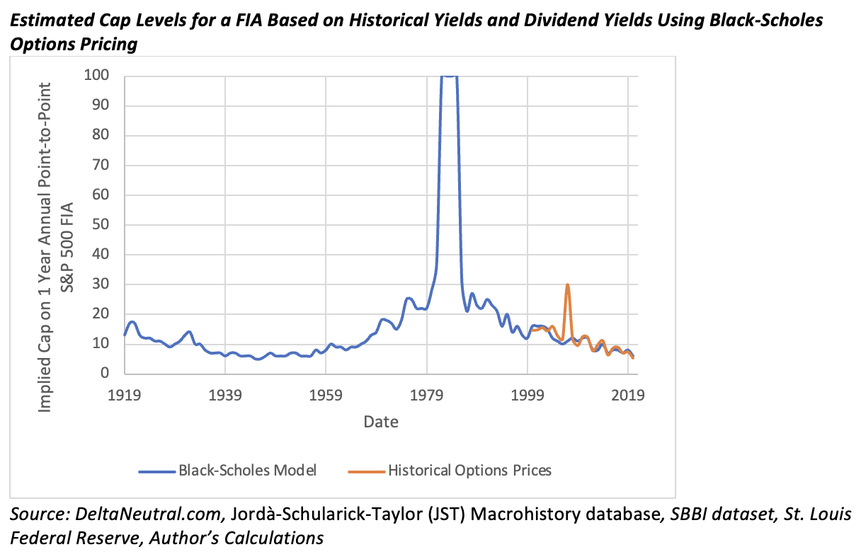
Estimated cap rates vary even more when the analysis is extended back to 1919. There would have been periods, for example in the 1980s, when the estimated cap rate would have been significant (easily exceeding 50%).

An important question for anyone who is using today’s cap rates with historical data is whether they would have been comfortable using the cap rates in the 1980s had a similar analysis been repeated then. Neither would be accurate because products would reflect circumstances, but they are relevant to investors historically.

Portfolio implications

Next, I attempt to determine the portfolio implications for using different cap models with a FIA.

This analysis is based on historical annual calendar returns from 1926 to 2020, where bonds are proxied by the SBBI Intermediate-term Government Bond Index and stocks are proxied by the SBBI Large Blend Index, which I refer to as the S&P 500 for simplicity purposes.

For the analysis, I estimate the returns an investor would have achieved in a hypothetical FIA using either the previously estimated caps, which evolved over time historically based on prevailing yields (called the adjusted model), or a constant cap rate for the entire period.

The constant cap rates reflect a model where caps are based on products that may have existed at a given point in time, where that level is then applied to all historical data. For example, the 5% cap is consistent with caps today; the 10% cap would have been appropriate around 2010, and the 15% cap would be appropriate in the mid-1990s. The credited return for the FIA is based on the price return of the underlying index, which is the S&P 500 (i.e., the SBBI Large Blend Index).

The table below shows the returns of the different investment strategies. No fees are assumed for any of the approaches.

The returns of the hypothetical FIA, with caps adjusted to reflect historical rate environments, is roughly consistent with a 20% equity/80% bond portfolio. It has similar volatility to the 20% equity portfolio, but significantly lower downside risk because the FIA is assumed to not have a negative return.

The return of the FIA is significantly less attractive with the constant caps, especially with a 5% cap, which reflects the current cap environment.

While FIAs are often noted as a “bond substitute,” their diversification benefits are generally less than those of bonds since their underlying return is based on the price return of stocks. For example, while the correlation between stocks and bonds has been effectively zero over the period, the correlation between the hypothetical FIA with adjusted cap and bonds has been approximately 0.3 and the correlation between the hypothetical FIA with adjusted cap and stocks has been approximately 0.7.

Next, I ran a series of portfolio optimizations to determine how the optimal allocations to the FIA would vary based on whether the caps are adjusted to account for historical conditions or based on a constant 5% cap.

The optimal portfolios are determined using a constant relative risk aversion (CRRA) utility function where the goal is to maximize the certainty-equivalent wealth given the respective risk aversion level based on the one-year returns. This approach captures the unique return distribution associated with FIAs, which have a relatively non-normal return distribution (e.g., it is not clear if a common metric like standard deviation would be appropriate). A cash proxy, which is the SBBI 30-day T-bill series, is also included in the analysis.

The results for seven risk aversion coefficients are included in the exhibits below.

The optimal allocation to the FIA is notably different for the two sets of optimizations. While neither FIA receives an allocation for the more risk tolerant levels (with a risk aversion coefficient of 2 or less), which is not surprising given the “lower risk” nature of the products, the allocations to the FIA increase as risk aversion increases when the cap is assumed to adjusted over time.

At the same time, the FIA never receives an allocation when a 5% flat cap is assumed. In other words, appropriately considering how caps would evolve over time can result in a meaningful allocation to a FIA, but using caps based on today’s yields (assuming historical returns) is unlikely to do so.

The difference in the relative efficiency between the two cap approaches is expected and demonstrates the significantly different perspectives on the efficacy of the products depending on which assumptions are used.

Conclusions

A model is only as good as its assumptions. Flawed assumptions will yield flawed outputs, an effect commonly referred to as, “garbage in, garbage out.”

Today’s low yield environment needs to be incorporated into financial projections, especially when determining the efficacy of an investment that is directly affected by low interest rates. For example, cap rates for one-year annual point-to-point FIAs on the S&P 500 with 100% participation rates should be approximately 2.5 times the yield on AAA bonds.

Annuities are not going to work for everyone, but it’s misleading to apply the current attributes of annuities (i.e., cap rates) in a purely historical context.

David Blanchett, PhD, CFA, CFP®, is managing director and head of retirement research at PGIM DC Solutions. PGIM is the global investment management business of Prudential Financial, Inc. In this role he develops research and innovative solutions to help improve retirement outcomes for investors.

Read more articles by David Blanchett