How Dedicated Portfolios Reduce Behavioral Risk

Dedicated portfolio theory versus modern portfolio theory

Most advisors are trained to look at asset allocation through the MPT lens. MPT assumes there is a valid way to determine a client’s “risk tolerance.” It then says to build a corresponding portfolio with X% in equities and Y% in fixed income, such as the classic 60/40 retirement portfolio. One should maintain that allocation by rebalancing periodically or when the proportions drift away from their targets by more than some amount, such as plus or minus 5%.

Can risk tolerance be measured? Are the questionnaires some advisors use valid? Psychometricians question it (Grable and Lytton, 1999; Roszkowski, Davey, and Grable, 2005; Grable, 2017).

There are significant differences between DPT and MPT. DPT focuses on building portfolios to generate a secure, predictable stream of future cash flows. The word “dedication” comes from the idea that the portfolios are assigned to producing those cash flows. This is the source of the institutional name “liability-driven investing.” Bill Sharpe calls it “cash matching” (Sharpe, Alexander, Bailey, 1995). For retirees, these cash flows will provide predictability and certainty to cover living expenses and other foreseeable items, such as car replacements, special vacations, grandchildren’s college expenses, etc. These are the sorts of details that advisors – at least good ones – typically build into a lifetime financial plan.

Predictability and certainty are achieved by purchasing individual bonds, holding them to maturity, and collecting coupons, principal and redemption payments for withdrawals. To minimize default risk, only investment-grade or government bonds are used. Returns may be low – these are fixed income securities – but security takes precedence.

Some may think bond funds would suffice. But, as mentioned earlier, bond funds may decline at the same time as stocks, providing no refuge for those who need to sell. Furthermore, they are not as predictable and certain as holding individual bonds to maturity. Bond funds behave more or less like sluggish stocks – they rise and fall. A portfolio of individual bonds held to maturity, on the other hand, may rise and fall, but these intervening evaluations are meaningless. All that matters are the coupon payments and redemptions. From the perspective of the financial plan, volatility of the fixed income allocation can be treated as zero. That is a fundamental and critical difference between DPT and MPT.

MPT makes no specification as to how the fixed income allocation is to be held. In a sense, MPT treats all fixed income investments alike – no distinction between individual bonds or bond funds. But when fixed income is dedicated to providing cash flows, the investor gets triple duty from the fixed income allocation – stability plus predictability plus certainty. This security is what makes DPT appealing to retirees when presented with it. It is perfect for the coronavirus scenario we are witnessing. And it is perfect for advisors who build individualized financial plans rather than the generic models that large brokerages require all their brokers to use.

Dedicated portfolio theory for personal financial planning

DPT can be best understood by examining four key elements that take it from theory to implementation and give clients peace of mind during markets like the March 2020 madness: the desired cash flow stream, the income portfolio, the growth portfolio, and the “critical path.”

1. Cash flow stream

DPT starts with identifying the stream of cash flows desired for the retiree’s life span. This requires serious, detailed planning. Specific cash flows for the projected withdrawals must be estimated for each year. Fortunately, most planning software generates this stream as a primary output. DPT’s goal is to provide these cash flows at minimum cost with the maximum probability of success for the duration of the plan. These withdrawal estimates can always be adjusted, of course, if circumstances change (divorce, death, inheritance, etc.).

2. Income portfolio

The individual bonds purchased and held to maturity become the “income portfolio.” This portion of the overall portfolio is dedicated to providing income over the specified time horizon. The planner can set a minimum and maximum length for this time horizon – five to 10 years is typical. But some prefer to extend to 15 to 20 years because none of the nine common domestic equity asset classes tracked by Morningstar (large value, large core, … small growth) have ever suffered a negative return rate over such long time horizons. This will be discussed in the growth portfolio section below.

Some might argue that determining length of horizon is as arbitrary as determining risk tolerance. There is no hard evidence to refute this argument. However, most people have better insight (at least not worse insight) as to the broad timeframe of secure income that would make them feel calm compared to how they would react to volatility, which can be either bad (down) or good (up).

The explanation for five to 10 years being most common may be that most people, especially retirees, are able to make some reasonably comfortable and accurate predictions about their lives that far into the future. It does not take much math to predict when your grandchildren will be headed off to college, when the next major anniversary will take place, etc.

The explanation may also stem from the fact that each year in the time horizon will require about 4% or 5% of the portfolio if the “four percent rule” for withdrawals is being followed, at least approximately. That means an eight-year horizon would require about 32% to 40% allocation to fixed income. In other words, an allocation of 32% to 40% would purchase about eight years of secure, predictable income at current interest rate levels.

The probability of success that a portfolio will last a lifetime based the historical record of returns tends to flatten out beyond about eight to 10 years. In fact, if too much is allocated to fixed income, the probability of success over 30 years will decline because of the lower returns. That is, if an acceptable probability of success and level of income can be attained within eight to 10 years, but longer horizons would entail a significant decrease in income to maintain the same probability of success, why extend?

To illustrate how DPT implementation works, consider two examples of cash flows a retiree might want: a regular “smooth” cash flow and an irregular “lumpy” cash flow. Both cases assume a starting portfolio of $1,000,000, an initial withdrawal of $40,000, eight years of secure income, and annual inflation protection of 3% per year, and the same total sum of withdrawals.

Example 1: Smooth portfolio withdrawals

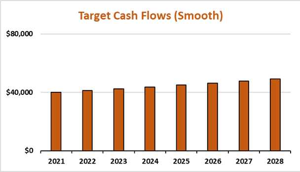
Exhibit 1A displays the regular, smooth series of withdrawals from an eight-year income portfolio starting at $40,000 in 2021 and increasing with 3% inflation from a $1,000,000 portfolio. In this case, the total cash flows would equal $355,693 over the entire time horizon (average $44,462).

Exhibit 1A
Target Cash Flows: Smooth Income Portfolio Withdrawal Stream

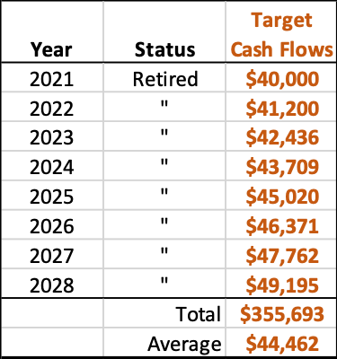
Source: Asset Dedication

The trick is to buy the bonds in just the right quantities and maturities so they exactly match the predicted future liabilities at minimum cost. Exhibit 1B illustrates the fixed income securities that would accomplish this. These were actual securities available at the time this example was constructed in March 2020, and used proprietary mathematical procedures to achieve minimum cost.

CDs comprise the first four years and federal agency bonds the last four. In this case, the agency bonds were both Federal Home Loan and Federal Farm Credit bonds. It is often the case that CDs pay higher rates than agency bonds for shorter maturities. But they are much scarcer for longer maturities. U.S. Treasury bonds would be the absolute safest and most liquid, of course, but CDs and agencies are both considered U.S. government--backed issues and carry higher returns. The higher returns are primarily a liquidity premium – they will be held to maturity, so why pay extra for unneeded liquidity?

Exhibit 1B
Fixed Income Securities Needed to Fund Smooth Withdrawal Stream

The cash flows have a 99.627% correlation with the target income stream. The fit cannot be perfect because bonds must be purchased in integer (whole number) lots (usually $1,000 or higher units). The overall difference, dollar-wise, is only -$583 (about $73 per year over the eight years) or about 0.16% (16 basis points) of the total income desired, $355,863. The total cost of the income portfolio is $339,778. When interest rates were more normal a few years ago (the rate on 10-year Treasury bonds historically back to 1800 was about 5%), the cost would have been lower.

Example 2. Irregular portfolio withdrawals

Sometimes, the withdrawal pattern over a time horizon will not be smooth in retirement. It will be irregular or “lumpy” due to long-awaited vacation cruises, car purchases, real estate sales, etc. It is the same total cash flow over eight years as Example 1, but the pattern is not smooth.

Exhibit 2A
Target Cash Flows: Irregular Income Portfolio Withdrawal Stream

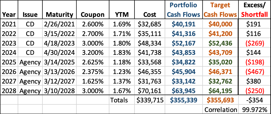
Exhibit 2B shows the correct portfolio using the same bonds but in different quantities. Note the different pattern of bonds needed in the cost column caused by the different pattern of cash flows needed. The total cost is nearly the same ($339,715). The correlation is even higher (99.972%). The total difference in dollar terms is also smaller, ($354, or about $44 per year over eight years), or 0.10% (10 basis points) of the total cash flow stream.

Exhibit 2B
Fixed Income Securities Needed to Fund Irregular Withdrawal Stream

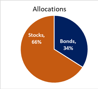
In both cases, the asset allocations are nearly identical: 34% bonds, 66% stocks (see Exhibit 3). That may sound a little aggressive for a retirement portfolio, but this portfolio provides eight years of predictable and certain cash flows regardless of what happens in the stock market. If a client were to ask, “Why do I have 34% in bonds?” the rational is easily explained, “Because you wanted eight years of secure income regardless of what happens in the market.” If they had wanted 10 years of protection, the allocation to bonds would have gone up to about 43%.

Exhibit 3
Asset Allocation for Both Examples

MPT does not offer such a direct linkage. Instead, its bond allocation is usually defended by saying it is based on the client’s responses to the risk tolerance questionnaire, where “risk” is defined as volatility. As mentioned earlier, many psychometricians have serious doubts as to its validity.

Most people define risk as running out of money, not the standard deviation of month-to-month portfolio values. This raises troubling questions about risk tolerance questionnaires. Many advisors still use them, but some admit they use them primarily to protect themselves, not because they believe them to be valid.

The allocation to bonds based on DPT is much more intuitive and transparent for most clients. And when people understand something, they are much more likely to rely on it, as is desperately needed at times like these.

At this point, it is common to ask about replenishing the portfolio as time passes. Bonds will mature to provide a year’s income, but the eight years of protection will now be down to seven years. Should the income portfolio be replenished by buying a new eight-year bond for the back end of the time horizon? The answer depends on where the overall portfolio stands relative to its long-term target. This will be covered in the section on the critical path below.

3. Growth portfolio

With DPT, bonds are dedicated to income, and equities are dedicated to growth. The growth portfolio’s purpose is to grow fast enough to replenish the income portfolio as its bonds mature each year. For example, if a client starts with an eight-year time horizon, one year later, only seven years of income remain sheltered in the income portfolio. If the client and planner agree they wish to maintain the original eight years of protected income, the planner must sell equities out of the growth portfolio to purchase a new eight-year bond.

The growth portfolio should integrate with the income portfolio by targeting the same time horizon. Theoretically, there should be growth portfolios targeting time horizons that exactly match the income portfolio time horizon. But it turns out that the difference between a portfolio designed for, say, eight years is not much different from one designed for nine years. The same is true for a 16- versus a 17-year portfolio. From a practical standpoint, different growth portfolios with only minor differences could lead to major administrative headaches.

To collect the time horizons into manageable groups, a statistical tool known as “cluster analysis” is needed. This tool delineates where to draw the lines so that the members within a cluster differ less from each other than from other clusters. Growth portfolios for 1-3 years, 4-6 years, 7-15 years, and 16-40 years using index and mutual funds are available from this analysis.

Another factor to consider is defining the goal of the growth portfolio. Most research into asset allocation focuses on attempting to maximize the expected return. But retirees are likely more on the conservative side. Thus, a better goal would be to use the “minimax” principle: find the allocation that maximizes the minimum return. With this strategy, all possible allocations are tested to see which one would lead to the highest return in the worst-case scenario for that time horizon. When the income portfolio needs to be replenished by sales from the growth portfolio, the chances are better that the sales will be at an opportune time. More on this in the critical path section below.

As might be expected, income portfolios with longer time horizons would have more aggressive, faster growing equities, which would have time to soften the impact of short-term volatility. Shorter income portfolios would have more stable, though slower growing equities. This is shown in Exhibit 4, taken from an article published last year, (Huxley and Burns, 2018), showing the dominance of small and value stocks over other asset classes as time frame grows ever longer (international and emerging market stocks were not part of that study). The longer the horizon, the greater the likelihood of positive results for all equity classes, and the more aggressive, the more so.

Exhibit 4
Average, Worst, and Best Performance for 1, 5,10,15,20, and 30 Year Holding Periods (Ending Year for Worst and Best), 1927-2017
Legend
Asset Classes: Value (V), Core ©, Growth (G), Large, Mid, Small

Source: Center for Research in Security Prices, (first published in Retirement Management Journal, Investment & Wealth Institute, Vol. 7, No. 1, 2018).

4. Critical path

As each year passes and a bond matures, the time horizon of the protected steam of income embedded in the income portfolio becomes one year shorter. An initial eight-year income portfolio will become a seven-year income portfolio one year later. The decision must be made, therefore, whether to roll the portfolio forward by buying another bond at the back end to maintain the same horizon.

Guiding this “roll-don’t roll” decision is the critical path analysis. It plots the path the overall portfolio should follow over the lifetime of the plan to achieve an acceptable probability of success in meeting all financial goals. It often stretches 30 years or more. It is plotted as the white dotted line in Exhibit 5 that separates the green safety zone from the red danger zone in a hypothetical example. The yellow line represents the value of the total portfolio at the end of each year.

To explain how this works, several years of fictional experience are illustrated in Exhibit 5. Assume an eight-year portfolio was constructed in mid-2020 with the first bond maturing at the beginning of 2021, and the last bond maturing at the beginning of 2028. As the yellow line illustrates, the portfolio fell below the critical path at the end of the first year. The portfolio has a less-than-acceptable probability of success. The decision therefore would be “don’t roll” at the end of 2021. That is, do not sell equities to replenish the income portfolio. Instead, let it ride for another year to see if the market turns around and the growth portfolio recovers. In this case, the income portfolio would contain seven instead of the desired eight years of protected income.

Exhibit 5
Critical Path

Source: Asset Dedication

At the end of 2022, when the income portfolio has six years of income remaining, market returns improved, boosting the portfolio back to its critical path. Thus, enough stocks were sold at the end of year 2 to roll the income portfolio out another year to cover 2029. The secure income stream is now seven years. Research has shown that selling enough to extend it back out to the original eight years all at once can harm the probability of meeting the long-term goals.

At the end of 2023, however, the market dropped, so the income portfolio again contained six years of income. As a result, the income portfolio again was not replenished.

At the end of 2024, when the income portfolio was down to five years, the market recovered and boosted the portfolio’s overall value back up to its critical path, so sufficient equities were sold to extend another year, with the last bond maturing at the beginning of 2030 (six years).

In the years following 2025, the fifth year of the original plan, the portfolio remains above the critical path. That means the growth portfolio will continue to be replenished yearly, maintaining the six years of protection at each renewal. If the portfolio rises to 20% or more above the critical path, the decision may be made to build a longer the income portfolio, extending it back out to seven, eight, or perhaps even nine, 10, or more years. In gambling terms, that is equivalent to taking the money off the table.

At some point, a client may decide that the income portfolio is as large as they think reasonable (say, 15 years), and simply keep it there, replenishing it only one year at a time to maintain it at a maximum of 15 years.

Bear markets can last longer than one year, of course. The longest on record was just under three years – 1929 to 1932 – the beginning of the Great Depression. Continuing to watch the time horizon of protected income dwindle in such a case may cause many clients to put a limit on how short the horizon will be permitted to go, such as five years. In this case, the minimum five-year horizon could be maintained by replenishing each year until the advisor has a chance to consult with the client about the need for making changes in the underlying financial plan in terms of spending, acceptable probability of success, etc.

In engineering terms, the critical path is the dynamic control mechanism for rebalancing the allocation of investments between bonds and stocks. The old MPT practice of rebalancing every year or whenever the allocations drift to far from their targets is gone. Rebalancing is now based on each client’s financial plan and its progress in meeting long-term goals. This is where rebalancing should have been all along.

Historical data allows estimates of the probability the portfolio will finish in the safety zone. Exhibit 6 traces the paths a portfolio could follow for the subsequent 30 years with this strategy if the client had retired in any of the 30 years from 1927 to 1989.

In this example, the portfolio failed only once – for someone who retired in 1929, the dawn of the Great Depression, when the portfolio would have lasted only 27 years (see blue line in Exhibit 6). This failure, however, is based on the unlikely assumption that the person would not change their spending habits even if they were below the critical path. Research suggests that if the portfolio falls below the critical path by more than 20%, the probabilities of success will likely drop below acceptable levels. The advisor would need to consult with the client about making changes in the parameters of the underlying plan.

Another axiom of MPT – volatility is risk – no longer makes sense for a portfolio in the safety zone above the critical path. Its fluctuations have little meaning unless they cause the portfolio to fall below the critical path.

Exhibit 6
Historical Audit Trails of Total Portfolio Values Over All 30-Year Spans Since 1927

Source: Asset Dedication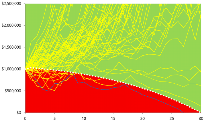

DPT performance

Aside from its historical performance, how does DPT compare with existing strategies in terms of meeting portfolio goals? Wade Pfau, a widely respected retirement researcher, concluded that retirement portfolios that utilize time segmentation based on DPT provided higher probabilities for long-term success (Pfau, 2017). Exhibit 7, taken directly from his article, demonstrates its superiority compared with a classic 60/40 portfolio based on MPT. The horizontal axis is the portfolio’s time horizon, while the vertical axis shows the probability of the portfolio lasting as long as needed. Clearly, the dedicated portfolio provides the best results.

Exhibit 7
Retirement Duration versus Probabilities of Success

Source: Wade Pfau, “Is Time Segmentation a Superior Strategy? Part 3,” Advisor Perspectives, April 3, 2017. Reproduced with permission.

Conclusion

Some might find it amusing that the term “modern” is still applied to a strategy born in the 1950s (Markowitz, 1952), but MPT certainly has had a good run and continues to serve as a great starting point for understanding the choices one must make when investing. But as its author, Harry Markowitz, has said, it was designed originally for institutional investors, not people (Markowitz, 1991). For retirees, DPT provides a more intuitive investment approach and better results.

More importantly, DPT provides another way for advisors to differentiate themselves from those who do not make planning the cornerstone of their practice. Most brokers, who may call themselves advisors, are likely to continue praising MPT. MPT was great for the giant Wall Street wirehouses because it provided the opportunity to follow the same model as fast-food restaurants, namely a fast, simple investment process:

1. Take the risk tolerance quiz.
2. You are this type of investor.
3. Invest X in stocks, Y in bonds.
4. Thank you. Next investor please!

It is unfortunate for the general public that while everyone recognizes that technology has improved, some pseudo-advisors are stuck in 1950s, at least when it comes to investment strategies.

Stephen J, Huxley, Ph.D., is a professor in the School of Management, University of San Francisco, co-founder and director of research, Asset Dedication LLC. Brent Burns is co-founder and president, Asset Dedication LLC. Jeremy Fletcher, CFA, is director of investments, Asset Dedication, LLC.

References:

Grable, J.E, and Lytton, R.H., 1999. “Financial risk tolerance revisited: the development of a risk assessment instrument,” Financial Services Review, Vol. 8, p. 163. doi.org/10.1016/S1057-0810(99)00041-4

Grable, J.E., 2017. “Financial Risk Tolerance: A Psychometric Review,” Research Foundation Briefs (CFA Institute), June 2017 Volume 4 Issue 1

Huxley, S.J. and Burns, B., 2018. “Visualizing U.S. Asset Class Returns Based on Time Horizons, Size, and Style,” Retirement Management Journal (Investment & Wealth Institute, formerly IMCA), Vol. 7, No.1, p. 46.)

Markowitz, H., 1952. “Portfolio Selection,” The Journal of Finance, vol. 7, no. 1, 1952, pp. 77–91., doi:10.1111/j.1540-6261.1952.tb01525.x.

Markowitz, H., 1991. “Individual versus Institutional Investing,” Financial Services Review, vol. 1, no. 1, 1991, pp. 1–8. doi:10.1016/1057-0810(91)90003-h.

Pfau, W., 2017. “Is Time Segmentation a Superior Strategy, Part 3” Advisor Perspectives, April 3, 2017

Roszkowski, M.J., Davey, G., and Grable, J.E., 2005. “Insights from Psychology and Psychometrics on Measuring Risk Tolerance,” Journal of Financial Planning, April, p. 66

Sharpe, W.F, Alexander, G.J., Bailey, J.V. 1995 “Investments” 5th Edition (Prentice Hall), p. 476.

Read more articles by Stephen J. Huxley, Brent Burns and Jeremy Fletcher