How to Make Time Segmentation Work in Practice: Three Options for Extending a Bond Ladder

Retirement-income bond ladders are divided between one-time and rolling ladders. One-time ladders are spent down over time. The bond ladder is not extended as bonds mature and it gradually disappears. These one-time ladders are not used with time segmentation strategies.

Our focus here is on rolling bond ladders, which are extended over time to keep the length relatively constant as time passes. They are not meant to be fully wound down. As bonds mature with the proceeds (face value and any coupon payments) spent for retirement needs, new bonds are purchased with other financial assets to extend the ladder length. Rolling ladders provide the basis for time segmentation strategies.

Rolling ladders can be designed to be automatically extended by one additional year as each year passes, or extended only when certain conditions are met. Possible decision criteria for extending a rolling ladder could be based on stock market valuations, interest rates, market performance or whether the individual is adequately funded as determined by a capital-needs analysis.

If a time segmentation approach does not offer clear rules for extending the bond ladder over time, then it is not a true retirement income plan that can be tested and analyzed. I will investigate three different methods for choosing when to extend the bond ladder as retirement progresses: automatic, market-Based, and personalized.

Automatic rolling ladders

Automatic rolling ladders, which Stephen Huxley and J. Brent Burns called “rolling horizon” in their Asset Dedication book, keep the same time horizon perpetually by automatically extending the ladder length each year as a bond matures. This is done for as long as the growth portfolio has sufficient assets to extend the ladder length. An initial ladder length is chosen and the ladder is built. At the end of each year, the ladder is extended by one year so that the length remains fixed over time.

This strategy involves taking ongoing distributions from the growth portfolio, which may be 100% in stocks or including some combination of other assets. The distribution amount is not the full value of spending, but rather the cost of the bonds to be purchased based on the then-prevailing interest rates. If and when the growth portfolio depletes, the ladder will continue to provide income without being further extended until it is wound down completely and all assets are depleted.

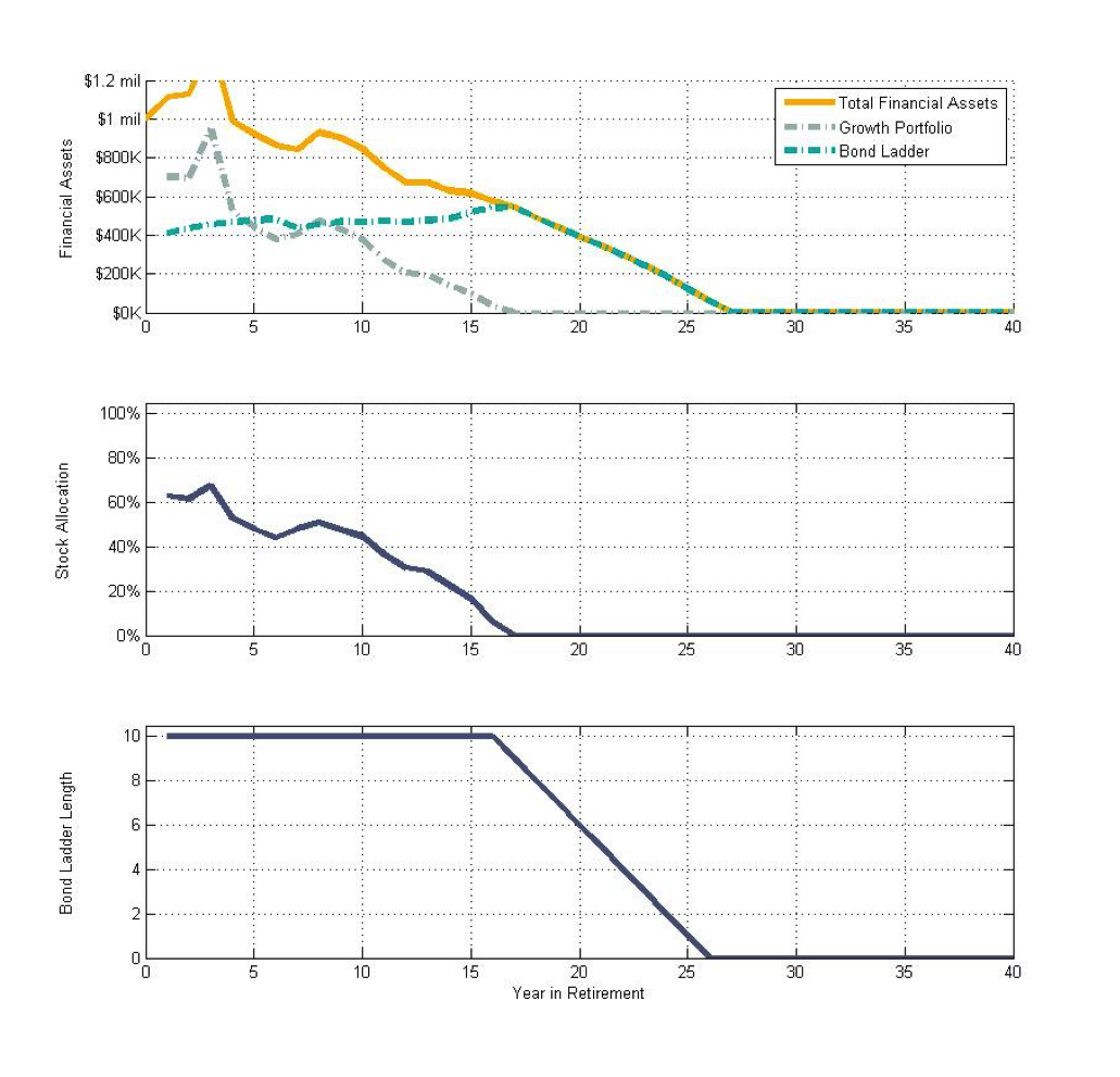
Figure 1 provides the outcomes for a Monte Carlo simulation for stock returns and bond yields to show how an automatic rolling ladder might perform in practice. This retiree seeks to support an initial $40,000 annual spending goal with an annual 2% cost-of-living adjustment for as long as possible in retirement. The retiree has $1 million at the start of retirement to divide between a bond ladder and a stock portfolio. The retiree seeks to maintain a 10-year bond ladder providing the desired annual spending throughout retirement. With a 2.45% initial bond yield and assuming a flat yield curve, building the initial bond ladder requires 39.2% of the asset base. The other 60.8% of assets are left in stocks. While I allow interest rates to fluctuate randomly over time, I simplified by assuming a flat yield curve. Relatively to an upward sloping yield curve, a flat yield curve lowers the costs of short-term spending and raises the costs of long-term spending. But these factors will tend to offset one another and with low interest rates the differing assumptions will lead to relatively minor differences in ladder costs.

In this single Monte Carlo simulation, a total-return investment portfolio that uses annual rebalancing to maintain a fixed 60.8% stock and 39.2% bond allocation would have supported spending until year 30 of retirement. With an automatic rolling ladder, wealth depletes in year 27. Because the growth portfolio experiences early losses, the automatic replenishing of the bond ladder each year pushes the stock allocation downward over time. In year 17, the remaining assets in the growth portfolio are transitioned to the bond ladder. At this point, the bond ladder can support nine more years of full income along with a portion of the tenth year’s income. Assets are fully depleted in year 27. Early stock losses raised the necessary distribution rate to support rebalancing, creating too much pressure on the growth portfolio. Time segmentation did not support a better outcome than a total-return portfolio.

Figure 1

One simulation for an automatic 10-tear rolling ladder

to support an initial $40,000 spending goal with a 2% COLA

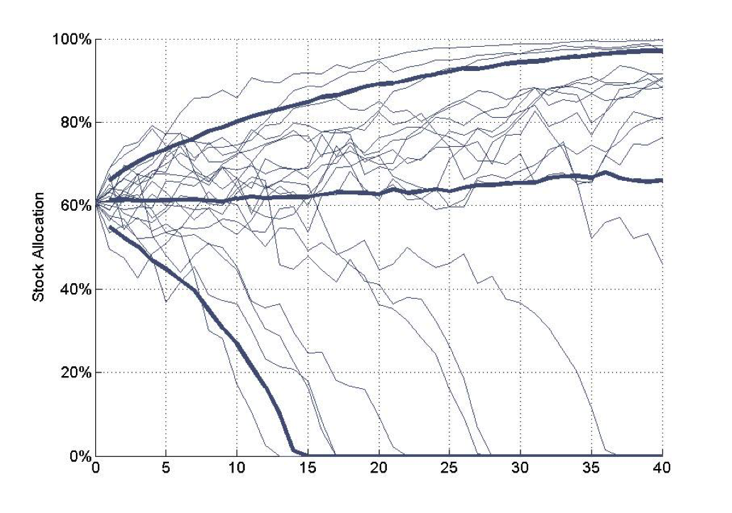
Next, Figure 2 provides a sense of the range of possibilities for the dynamic asset allocation generated by 10-year automatic rolling ladders. Twenty random simulations are shown with thin lines, along with the 10 th, 15 th, and 19th percentiles across the distribution using 10,000 Monte Carlo simulations. The median stock allocation stays relative close to its initial level with only slight upward drift. At the 10 th percentile, the stock allocation falls dramatically as the growth portfolio is spent down to extend the bond ladder over time. The growth portfolio depletes by year 15. On the other hand, the growth portfolio grows dramatically at the 19 th percentile, so that the stock allocation continues rising even as the bond ladder extends. This rising equity glidepath is triggered by strong stock market performance increasing the growth portfolio at a rapid pace that exceeds the distributions needed to keep the bond ladder fully funded.

Figure 2

Dynamic asset allocation in retirement

Twenty random simulations for an automatic 10-year rolling ladder

along with the 10th, median, and 90th percentiles for the entire dDistribution

Market-based rolling ladders

Market-based and personalized bond ladders are part of the category that Huxley and Burns call “flexible horizons.” Market-based rules for extending the ladder could be based on triggers such as positive stock growth, high stock market valuations or high interest rates. Noting whether the portfolio has grown is an objective criterion, but there is a degree of subjectivity involved in deciding whether stock market valuations or interest rates are high. It is important not to fall into the trap of using market timing to make these decisions and of using an ad hoc approach to ladder extension.

For an example of a market-based approach, I will use a rule that is similar to how the life insurance industry describes the use of cash-value life insurance and how Barry and Steven Sacks decide when to draw from a reverse mortgage line of credit. That is, if the stock market produced a negative return in the previous year, then the bond ladder is not extended in the current year. If the stock market produced a positive return in the previous year, then the ladder is extended to the full targeted length as long as there are sufficient assets in the growth portfolio to achieve this. For example, if the target ladder length is 10 years, then two years of negative returns would reduce the ladder length to eight years. If a positive return is experienced in the third year, then the ladder is extended by three years to account for that year’s spending and the two years that the ladder was not extended, in order to get back to the desired 10-year target length. If the growth portfolio fully depletes, the ladder is no longer extended and retirement income ends once the ladder reaches its final maturity.

Figure 3 provides the outcome for the market-based rolling ladder for the same Monte Carlo simulation used previously. In this case, we can see that until year 21, there are cases where the ladder length is allowed to decrease after years of negative stock returns. This slows down the pace of the reduction in the growth portfolio. However, the growth portfolio also depletes in this scenario in year 21. Then the bond ladder begins to wind down and assets are fully depleted by year 30. This market-based ladder provides slightly less total spending than could have been achieved with the fixed 60.8/39.2 asset allocation total-return portfolio, since less of the year-30 spending goal can be met. But compared to a total-return portfolio that used the same dynamic asset allocation as this market-based strategy, the bond-ladder version did perform slightly better. The total-return version with an ongoing matching dynamic asset allocation could have only supported the same income into year 29.

Figure 3

One simulation for a market-based 10-year rolling ladder

to support an initial $40,000 spending goal with a 2% COLA

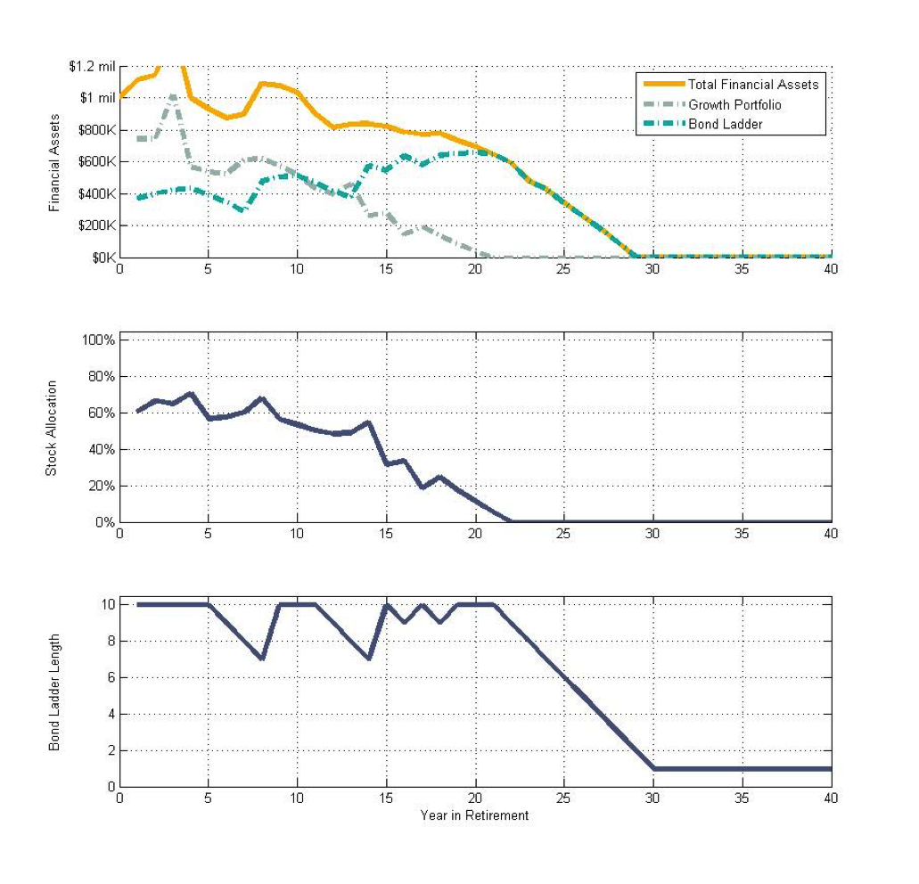
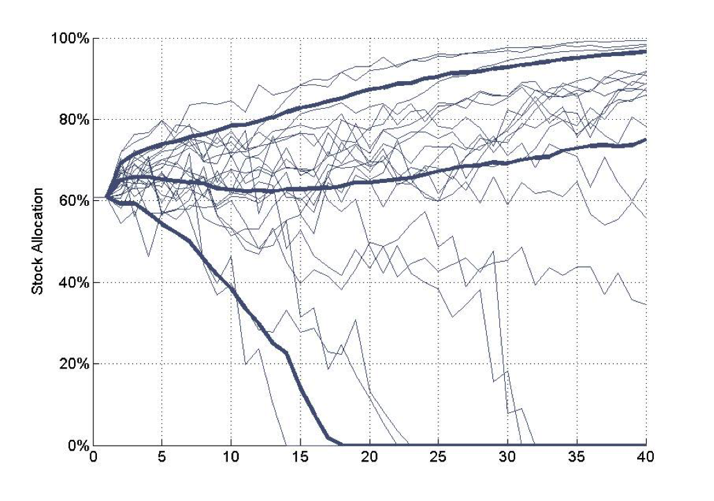
Figure 4 illustrates the range of possibilities for the dynamic asset allocation generated by the market-based 10-year rolling ladder. Again, 20 random simulations are shown with thin lines, along with the 10th, 50th, and 19th percentiles across the distribution. The pattern of asset allocation is similar to before, though the median stock allocation does rise more quickly to about 75% by the end of the time horizon. The ability to let the bond ladder decrease after a stock decline does help to preserve the portfolio a bit longer than otherwise, while also increasing stock allocations slightly compared to the automatic ladder. Again, effort is made to preserve the bond ladder length as much as possible, which does lead the stock allocation to decline after bad market outcomes. This happens at a slower pace than before, though, as the market-based approach provides more flexibility for short-term bond ladder reductions as well.

Figure 4

Dynamic asset allocation in retirement

20 random simulations for a market-based 10-year rolling ladder

along with the 10th, median, and 90th percentiles for the entire distribution

Personalized rolling ladders

Personalized rules are part of the family of variable spending strategies for retirement. They can be based on a “critical path” for retirement wealth. Within retirement-income planning research, I have observed three cases in which a “critical path” is used to help guide decisions around retirement spending. First, Huxley and Burns used a critical path to help decide when to extend the bond ladder in their Asset Dedication book. Second, a team of researchers at Texas Tech University used a critical path to determine when to take distributions from an investment portfolio and when to take distributions from a reverse mortgage line of credit. I discussed that method in my book, Reverse Mortgages: How to Use Reverse Mortgages to Secure Your Retirement. Third, David Zolt used the critical path to decide whether or not a retiree should take a full inflation adjustment for spending during each year of retirement.

The “critical path” helps to determine if the portfolio is on target to meeting the retirement goal. First, a retiree determines an end goal for the portfolio in terms of how long the portfolio should last, as well as how much spending it should support. Examples of portfolio end goals could be to deplete the portfolio by age 105, to maintain $100,000 at age 90, and so on. Next, these numbers are combined with the current portfolio value to determine a portfolio return assumption that will allow the end goal for the portfolio to be met. Third, this information is combined to determine a glide path for the value of remaining wealth throughout retirement, showing the wealth needed to remain precisely on track to meet the spending and portfolio end value goals. The critical path compares where the portfolio is and where it should be in dollar terms to be on track.

Volatility is not an appropriate measure of risk for personal financial planning. When one is in the safety zone above the critical path, volatility may not be risky, but a low volatility portfolio may be quite dangerous when one has fallen below the critical path and the portfolio is plummeting toward zero. The real risk in personal finances is if the wealth level falls below the critical path. In a sense, high volatility when above the critical path is less risky than low volatility when below the critical path.

Figure 5 provides an example of a critical path for retirement wealth. This individual has $1 million at retirement. She seeks to support $40,000 of spending with a 2% COLA for a 45-year retirement period. Wealth is allowed to be depleted at the end of 45 years. She determines that a 5% return is needed to support this retirement spending goal with her portfolio. The exhibit tracks the path of her remaining wealth with a 5% return to let her know where she should be during each year of retirement to be on a sustainable path toward meeting her retirement goal. Wealth above the glidepath represents a safety-zone, while retirement is in more dangerous territory if wealth falls below its critical-path value.

Figure 5

Critical path for sustainable retirement wealth

to support an initial $40,000 with a 2% COLA for 45 years

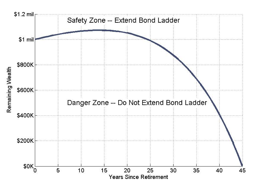
In each year of retirement, the retiree can compare the current value of her remaining wealth to the critical path value for her wealth. If her actual wealth exceeds the critical path, then she is in good shape with extra discretionary wealth. However, when her actual wealth falls below the critical path, she is falling behind in terms of being able to meet her full retirement goal. In the context of this discussion, the bond ladder can be extended further when wealth is above the critical path, but the ladder is not extended during years that wealth falls below the critical path. One instead relies on growth assets to recover and get back above the critical path before extending the bond ladder.

This action is designed to relieve the stress on the growth portfolio and allow it a better chance to recover before taking further distributions from it. It is predicated on faith in “stocks for the long run.” Unlike the other two ladder extension strategies, this one moves the portfolio toward 100% stocks when the portfolio is in danger.

Figure 6 provides the outcomes using a critical path approach to bond-ladder extension based on the same Monte Carlo simulation as used previously. In this case, we can observe that remaining financial assets quickly fall below the glidepath threshold, leading the bond ladder to be less than 10 years for much of the retirement period. The bond ladder dissipates by year 13 of retirement as the critical path threshold for extending the ladder is not passed again after the fourth year. Unlike the other strategies, this pushes asset allocation in the growth portfolio to 100% stocks as the bond ladder depletes. To illustrate the growth-portfolio depletion, I show that the asset allocation drops to 0% stocks once no assets remain. For this simulation, retirement spending was fully supported for 30 years, and the growth portfolio is depleted in year 31.

Figure 6

One simulation for a personalized 10-year rolling ladder

to support an initial $40,000 spending goal with a 2% COLA

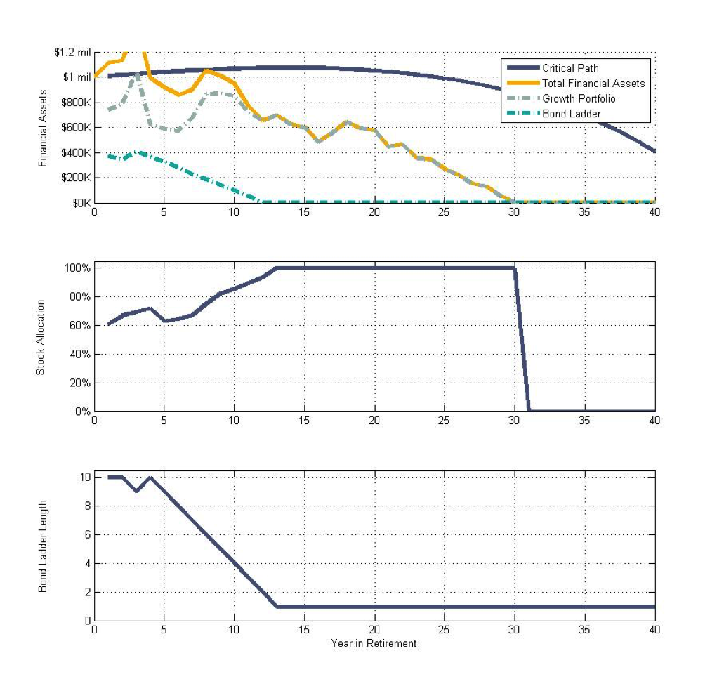
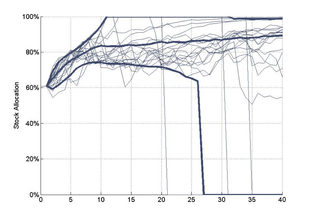
Figure 7 provides the corresponding analysis showing the distribution of the asset allocation over time, along with the stock allocation paths for 20 random simulations. We can observe clearly how this strategy pushes the stock allocation higher than the other strategies, since it leads to the bond ladder depleting prior to the growth portfolio. The stock allocation at the 10th percentile rises almost immediately as well, unlike in the other cases. The median stock allocation continues to rise, surpassing 80% within the first 10 years of retirement.

Figure 7

Dynamic asset allocation in retirement

20 random simulations for an automatic 10-year rolling ladder

along with the 10th, median, and 90th percentiles for the entire distribution

The bottom line

We have explored how three viable approaches for bond ladder extension work in practice. This is an essential ingredient for quantifying the value of time segmentation strategies. The final step, coming in part 3, is to test time segmentation strategies against total-return investment strategies.

Acknowledgements: I am grateful for helpful feedback on earlier drafts of these columns from Stephen J. Huxley and J. Brent Burns of Asset Dedication.

Wade D. Pfau, Ph.D., CFA, is a professor of retirement income in the Ph.D. program in financial services and retirement planning at The American College in Bryn Mawr, PA. He is also a principal and director at McLean Asset Management and the Chief Planning Scientist for inStream Solutions. He actively blogs at RetirementResearcher.com. See his Google+ profile for more information.

Read more articles by Wade D. Pfau