The Importance of Actively Adjusting RILA Account Allocations

There are two main RILA strategies: buffer and floors. With buffer products, some of the loss is absorbed first by the product, based on the buffer level; the investor suffers any loss beyond that point. For example, if the buffer is 10% and the return of the underlier is -40%, the annuitant would lose 30%. If the return of the underlier is negative, but not less than the buffer, the investor return would be 0%. With floor products, the downside is limited to a stated percentage, such as 10%. For example, if the floor is 10%, you can’t lose more than 10% regardless of the return of the underlier (e.g., the S&P 500). A RILA (or ETF) with a 0% floor would have the same risk profile as a FIA.

There are two primary ways returns are credited in RILAs, based on the participation (par) rate and a cap. The participation rate is the percentage of the underlier return that will be credited for the strategy. For example, if the participation rate is 50% (100%) and the market goes up 20%, you would earn 10% (20%). The “cap” is the maximum possible credited return. For example, if the cap is 10%, and the return of the underlier is 20%, only 10% would be the assumed return. According to data from LIMRA, 87% of RILA sales are in buffers versus only about 10% in floors, so buffers are definitely more popular among the two. The participation and cap rates are based on the return of the underlying index exclusive of dividends (i.e., the based on price only).

RILA terms (maturities) are shorter than FIAs. According to LIMRA’s 2022 Registered Index-Linked Sales Report, 99% of RILAs have terms that are six years or less, while only 15% of FIAs have terms less than six years. Living benefits are still relatively rare among RILAs, but interest is increasing.

The S&P 500 index is most often used in RILAs, and that has been constant over time. The exhibit below demonstrates this effect using data from Wink, where the S&P 500 index was selected for approximately 75% of RILAs but only about 40% of FIAs.

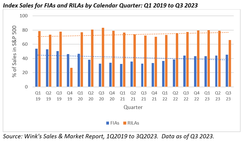
But the S&P 500 is rarely the only option available in RILAs. Many contracts have five or more options available; the high utilization is an active choice among advisors.

Two potential reasons for the lack of diversification of index strategies within RILAs are complexity and choice overload. Most financial advisors using RILAs likely do not have modeling tools to determine optimal allocations given the complexity of modeling RILAs (e.g., the returns are not normal). With RILAs, caps are constantly being adjusted based on market conditions (e.g., as interest rates change and valuations evolve), which leads to opportunities to adjust allocations to index strategies over time.

While there are a few tools available, they typically define risk as standard deviation and use historical returns, two assumptions that are suboptimal, something I explore in the next section.

Optimal RILA account allocations

When determining the optimal allocations using options, it is important to model unique return distributions of the product. Common risk metrics, like standard deviation (or variance), do not adequately capture the risk profile of buffered strategies, especially the nonnormal aspects of the return distribution.

This effect is demonstrated in the exhibit below, which includes the return distribution for an index (e.g., the S&P 500) with an assumed price return¹ of 7% with a standard deviation of 15% for a 10% buffer RILA.

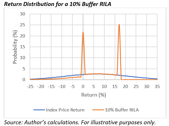
There is a high likelihood that the credited retutn of a RILA over a one-year period will be zero (within the buffer zone) or at or above the cap. This creates a unique return distribution (it looks like Batman’s mask) that is unlikely to be appropriately captured with basic risk definitions like standard deviation.

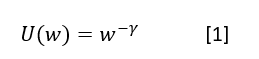
To account for the nonnormal returns associated with RILA, optimal portfolios are determined using a constant relative risk aversion (CRRA) utility function. Its goal is to maximize the certainty-equivalent wealth given the respective risk aversion levels, assuming a one-year investment period, as noted in equation 1:

Utility-based methods offer considerable flexibility compared to more traditional approaches, since they can “score” different parts of a distribution. CRRA is broadly used in academic literature.

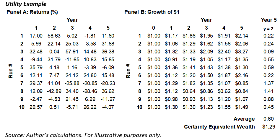
The exhibit below provides an example of the utility function in practice. It show a scenario with 10 runs that each last five years, where the target wealth value is the terminal value at the end of year five. The returns were randomly generated assuming an average return of 10% and a standard deviation of 20%. The values in year five were each raised to the assumed risk aversion level (y), which is 2 in this example. In the first run, the ending balance is $2.14 and $2.14^-2 = $.22. The average utility across the 10 runs is .60 and the certainty equivalent wealth value would be $1.29. If multiple asset classes were included, their optimal weights would be those that maximize the average utility of wealth across the total number of runs.

When determining optimal allocations, it is important to use expected, not historical returns. There can be notable differences between the two. The next exhibit contrasts the historical rolling annualized 10-year price returns for the S&P 500, the Russell 2000, and the MSCI EAFE indexes from Q2 2021 to Q4 2023 and expected returns (capital market assumptions, or CMAs) at different points in time, obtained from PGIM Quantitative Solutions.

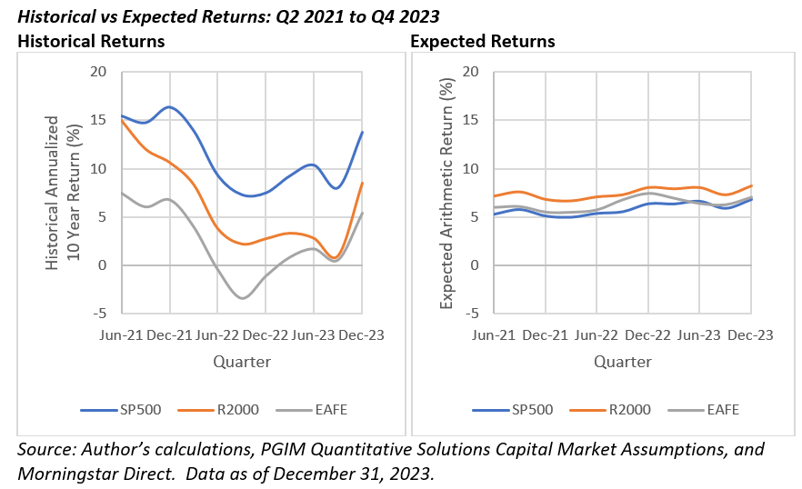
While the expected returns are consistent over time, they change slightly based on valuations. The differences are less extreme than the historical averages. For example, the 10-year price return for the MSCI as of December 31, 2022, was -1.06%. If this was the assumed return for optimization, the weight to any crediting strategy for that index would likely be zero. That is why it is prudent to use historical returns given the instability in the estimates.

The analysis used historical expected annual arithmetic returns to determine optimal portfolio weights. Standard deviations and correlations are constant for the S&P 500, the Russell 2000, and the MSCI EAFE at 15%, 20%, and 16%, respectively. Correlations can be obatined by contacting the author.

For this analysis, historical caps were obtained for a single RILA actual product focused on three indexes: the S&P 500, the Russell 2000, and the MSCI EAFE with two buffer levels: 10% and 15%, for a total of six possible options (but most RILAs have more options).

Caps are available from June 30, 2021 to December 31, 2023 and were reviewed on a quarterly basis. The available caps are included in the following two exhibits. The first set includes the actual caps by index for the 10% and 15% buffer levels and the second set includes the differences in the caps when compared to the S&P 500.

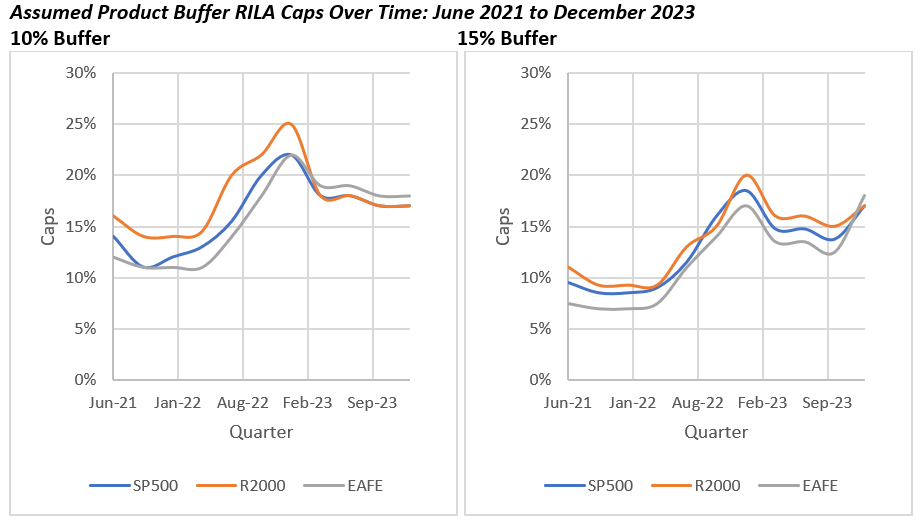
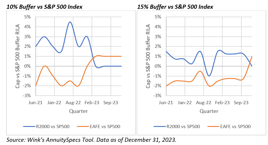
The first set demonstrates that the caps changed over time, in particular rising in response to the increase in interest rates that took place in 2022. The second set demonstrates there were variations among the respective indexes over time as well (i.e., their relative attractiveness changed).

The maximum assumed allocation to any of the six crediting strategies is 50% to ensure diversification. No fees or taxes were considered for this analysis. I performed 11 optimizations, one for each quarter from June 2021 to December 2023.

Optimization results

The next exhibit includes the optimal weight to the six crediting strategies for the 11 periods reviewed.

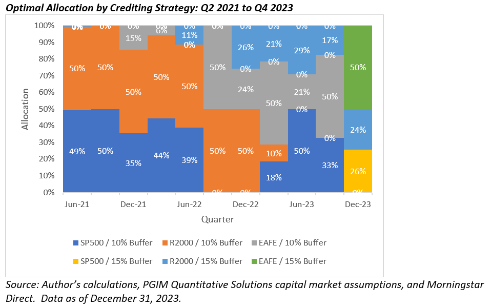
The optimal allocation varied materially over time, both in terms of the index as well as the buffer level.

The S&P index received a 31% allocation, on average, while the average allocation to the Russell 2000 was 45% and 24% to the MSCI EAFE. The 10% buffer was favored, receiving an average allocation of 81%. If a higher risk aversion were used, the allocations to the 15% buffer would have been higher, on average, but the allocations to the 15% buffer increased over the period. Overall, the analysis shows the optimal allocation to the available index strategies changes over time.

Next, I estimated the expected benefits of using the optimal strategy for an S&P-only approach (where there is an equal allocation to the 10% and 15% buffers for the S&P 500 index) versus an equal weight to the six available strategies. The alpha was determined by subtracting the certainty equivalent wealth from the optimal strategy to the two other options and the values for each period are included in the exhibit below.

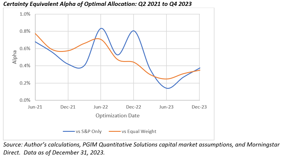
Both average expected alphas were approximately 50 bps historically, although that declined over time. Regardless, an average expected alpha of 50 bps is significant, and the benefits are likely to be materially higher if all the available crediting strategies available were considered.

Conclusions

Options are complex and embedding them in financial products has the potential to improve outcomes for investors but may introduce complexity that cannot be fully modeled by most advisors. This analysis suggests that determining optimal account allocations within a RILA can increase expected risk-adjusted returns. To the extent RILAs continue to gain interest and assets among consumers, information or tools will be necessary to ensure investors have the best expected outcomes possible.

David Blanchett, PhD, CFA, CFP®, is managing director, portfolio manager and head of retirement research at PGIM. PGIM is the global investment management business of Prudential Financial, Inc. He is also an adjunct professor of wealth management at The American College of Financial Services and a research fellow for the Retirement Income Institute.

¹ Credited returns in RILAs are generally on the price return of the index (exclude dividends).

A message from Advisor Perspectives and VettaFi: To learn more about this and other topics, check out some of our videos.

Read more articles by David Blanchett