Monte Carlo projections have become the popular way to do financial projections among advisors. Indeed, approximately 80% of financial advisors noted using the tool in a recent Alliance for Lifetime Income survey.
One common criticism I hear from advisors about Monte Carlo (especially from those who don’t use it) is that it incorrectly assumes returns are normally distributed (i.e., follow a perfect bell curve). But concerns around nonnormal returns and Monte Carlo are a red herring (i.e., nonissue) for a variety of reasons.
Perhaps most importantly, it is possible for a return distribution to be nonnormal in a Monte Carlo projection; its whatever distribution is assumed by the user or respective tool. While return distributions may not be perfectly normal at relatively high frequencies (e.g., daily), return distributions become increasingly normal over longer periods (e.g., annually). Finally, financial plans require a significant number of other assumptions that will have a materially greater effect on the outcome (e.g., saving, spending, length of retirement, etc.) than the specific moments of the return distribution of the opportunity set of asset classes.
The next time someone suggests that nonnormal returns are a problem with Monte Carlo, tell them that their concern is a nonissue!
Monte Carlo does it all
Monte Carlo projections are used by financial advisors to illustrate the uncertainty associated with accomplishing various financial goals, such as retirement. For example, in a recent survey I conducted with Prudential Financial, Inc. in February 2023 among 190 financial advisors, 80% of respondents noted using Monte Carlo, a nearly identical percentage as the advisors who noted doing so in the latest Alliance for Lifetime Income 2023 Protected Retirement Income and Planning (PRIP) Study.
The key differentiator with a Monte Carlo projection versus other projection methodologies (e.g., time value of money calculations) is the element of chance (i.e., randomness). Typically, forecasted returns are the only random (or stochastic) variable in financial planning programs that employ Monte Carlo; but other variables (e.g., age of death, age of retirement, etc.) could be randomized as well.
Financial advisors correctly say that Monte Carlo assumes returns are normally distributed. But the assumptions in a simulation are whatever the user, or creator of the program, specifies. In other words, the shape of the return distribution for the opportunity set of asset classes included can be whatever the respective user wants or tool allows (i.e., returns don’t have to be assumed to follow a normal distribution or bell curve).
Many (perhaps most) financial planning tools assume that returns are normally (or lognormally) distributed; that’s a choice that particular tool is making and is not a condition of a projection. While this distinction between Monte Carlo itself and the tools that use it might seem minor, if an advisor is especially concerned about assuming nonnormality, there are tools that can incorporate this.
Levels of nonnormality
Return distributions are generally described by four moments: the mean or average (first moment), standard deviation (second moment), skewness (the third moment), and kurtosis (the fourth moment). Concerns around nonnormality are typically related to the third and fourth moments, especially concerns that “bad outcomes” (i.e., significant negative returns) happen more frequently than implied by a normal distribution (i.e., standard deviation alone).
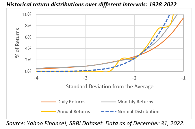
While there are a variety of statistical tests you can use to estimate how “normal” a given distribution of returns might be (e.g., the Shapiro-Wilk test), a straightforward approach is to compare the actual (historical) distribution of returns to a normal distribution and see how they differ. I do this using historical daily, monthly and annual returns for the S&P 500 from 1928 to 2022 (inclusive) in the exhibit below.
I focused on negative returns (i.e., the left tail of the distribution) since those are the returns that would be considered risky. Daily return data are obtained from Yahoo Finance!, while the monthly and annual data are from the Ibbotson SBBI series. For reference purposes, the average daily, monthly and annual returns were 0.03%, 0.93% and 11.75%, respectively, and the standard deviations were 1.20%, 5.41% and 19.71%, respectively.
The exhibit includes the percentage of the returns that are equal to or below the respective standard deviation value. If the point on the line for the respective historical times series is above the normal distribution line, it means the returns have occurred more frequently than implied by a normal distribution and vice versa.
While the historical return distributions were approximately normal, there were differences. For example, approximately 2.3% of all returns should be two standard deviations or more away (above or below) from the mean. Surprisingly, the historical return distributions were quite similar to this expected value, with the daily, monthly and annual values being 2.6%, 2.4% and 2.2%, respectively.
It’s the more extreme outcomes where the normal distribution appeared to fall apart for the higher frequency time series (e.g., daily and weekly). For example, only approximately 0.1% of all returns should be three standard deviations or more away from the mean; but the percentages were 0.9%, 0.8%, and 0% for daily, monthly, and annual, respectively. In other words, while annual returns were approximately normally distributed, when focusing on the likelihood of incurring large losses, higher frequency returns have been much riskier than implied through standard deviation alone (i.e., assuming normality).
Is the nonnormality exhibited in historical stock returns an issue? It can be from an investment perspective, especially for investors who have to price risk daily (e.g., investment banks) and therefore could impact the riskiness of a client portfolio (i.e., affect risk tolerance). But since financial plans last decades, the impact of nonnormality is relatively insignificant, especially in light of the other assumptions, which I discuss in the next section.
Estimation error is everywhere
Predicting the future, as they say, can be difficult. Any financial projection inherently relies on a number of assumptions, which are going to be wrong to varying degrees. The existence of estimation error is important since it places the importance of different assumptions in context. For example, the uncertainty around when someone is going to retire, how long they are going to live in retirement, how much they spend in retirement, whether they have a significant medical event, etc. is going to have a much larger impact on a financial plan (i.e., projection) than whether it’s possible to perfectly predict the exact return distribution.
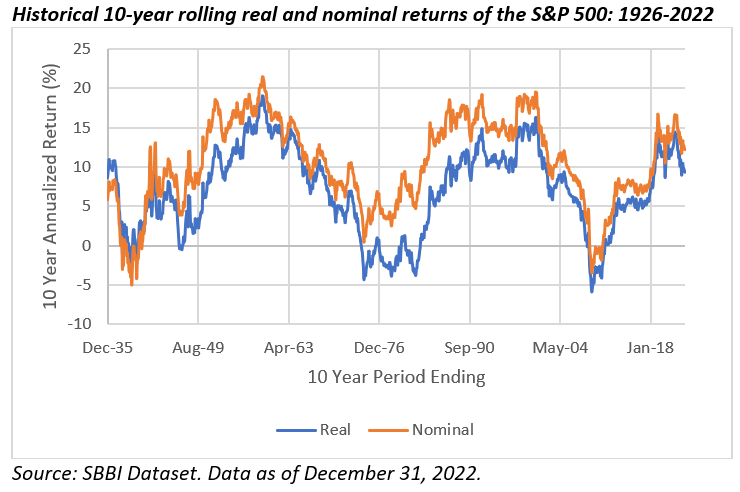
Even projecting returns (i.e., the first moment of the distribution) is difficult, as has been the case notably over time. The impact of low returns early in retirement has been well documented (i.e., sequence risk), and as the exhibit below demonstrates, there have been 10-year periods when stocks have done exceptionally well and poorly.
While the likelihood of experiencing these negative returns can be captured in the return distribution (i.e., forecasting skewness and kurtosis), each person will only experience one retirement (i.e., their unique “run” or “trial”). Correctly forecasting the mean return (which is impossible) is far more important than the additional return moments. Therefore, the precise shape of the return distribution of the asset classes included in a projection are relatively insignificant considering the other required assumptions.
Conclusions
Monte Carlo projections are an incredibly valuable planning solution, not because the projection itself is likely to be especially accurate, but because it provides a framework to create expectations for clients that can be adjusted over time.
Any financial projection, especially one spanning decades, will be “wrong” to some extent. To suggest that Monte Carlo is somehow not valuable, though, because it doesn’t incorporate nonnormal return distributions is not only factually incorrect (Monte Carlo can incorporate this), but it ignores that even the most basic assumptions in any plan are unlikely to hold.
While the efficacy of each Monte Carlo projection will vary based the quality of the assumptions, worrying about nonnormal returns is not where we need to spend our energy. There are other things that should be improved that are going to have a much bigger impact, such as personalizing client longevity assumptions, moving away from outcomes metrics like the probability of success, and better modeling of retiree liability (e.g., into needs and wants).
David Blanchett, PhD, CFA, CFP®, is managing director and head of retirement research at PGIM DC Solutions. PGIM is the global investment management business of Prudential Financial, Inc. He is also an adjunct professor of wealth management at The American College of Financial Services and a research fellow for the Retirement Income Institute.
A message from Advisor Perspectives and VettaFi: To learn more about this and other topics, check out our full schedule of upcoming CE-approved virtual events.
Read more articles by David Blanchett
 Monte Carlo projections have become the popular way to do financial projections among advisors. Indeed, approximately 80% of financial advisors noted using the tool in a recent Alliance for Lifetime Income survey.