In my previous series of articles (here, here and here), I explored the potential benefits of an emerging type of longevity solution, called a protected lifetime income benefit (PLIB), based on previously released research. A PLIB differs from a GLWB because the income changes are materially different and can decline. The PLIB concept is not new, with tontines being one of the earliest examples of products that provide protected lifetime income with a form of “shared” risk exposures.
The unique structure of PLIBs requires a different way of thinking about risk. With a GLWB, the annuitant should take on the maximum allowable risk level, an objective that is unambiguous. But the optimal risk level for a PLIB is less clear, given the downside exposure with negative returns.
This piece explores the optimal risk level for PLIB strategies. Overall, more balanced risk strategies in PLIBs are likely to be optimal (e.g., 40-50% equities), although the ability to personalize the risk level is important based on the household situation and preferences.
PLIB mechanics
Payouts from PLIBs are similar to GLWBs, which were covered in-depth in the first piece in the series but are reviewed again here. PLIBs provide some guaranteed income for life regardless of the underlying account value (i.e., even if it goes to zero). The key difference is that the income from the PLIB changes over time based on performance (investments and/or mortality, depending on the structure), while the income from a GLWB is based on adjustments to the benefit base. For GLWB income to increase in the distribution phase, the return must exceed the distribution amount and fees, something that is increasingly unlikely over time.
The growth in PLIB income is typically based on the credited return minus any applicable fees (i.e., net performance), although gross performance could also be used (ignoring any mortality adjustments). For example, if the income from a PLIB was $5,000 and the net return of the account (including fees) for the prior period was 20% the income level would increase by 20% to $6,000. In this case, the income would increase regardless of the underlying value of the contract.
Since the PLIB payout is solely focused on returns (this analysis excludes mortality), the probability of an income increase is significantly higher with a PLIB than a GLWB; however, the reverse is also true, whereby the income from a PLIB can decline if the returns are negative (while they would not for a GLWB). For example, if net return of the PLIB account was -20%, an income of $5,000 would drop to $4,000. The income could drop even further depending on account performance.
This creates an important dynamic around the optimal risk level for PLIBs, which I address in this piece.
The income level from a PLIB can either remain constant (for the life of the annuitant) once the account has been depleted or continue to evolve based on the performance of the account. For this analysis, I assumed the income is based on the previous year’s value before the account is exhausted.
The optimal strategy
I determined the optimal retirement income strategy based on the constant relative risk aversion (CRRA) utility function, shown in equation 1, where the amount of utility (U) received varies depending on level of consumption (c) and level of investor risk aversion (γ).

I used a utility-based approach, versus other metrics more commonly used by financial advisors such as the probability of success, since it better captures the economic implications of shortfall in retirement. Implied within the CRRA utility function is the law of diminishing marginal utility, whereby negative outcomes (especially extreme negative outcomes) are weighted more heavily than positive outcomes. The specific utility approach I used in this research is a modified version of the approach introduced by Blanchett and Kaplan (2013). Please refer to the main paper, in particular Appendix 1, for additional information on the model.
The analysis assumes the household is a male and female couple, both age 65, retiring immediately with $500,000 in savings. The savings assumed for the analysis is not that important; rather it is the savings relative to other sources of retirement income assumed. Taxes are ignored for the analysis.
I assumed the PLIB has a 4.0% initial payout rate with a 1.5% total annual fee. Income from the PLIB changes based on account performance, which is reduced by the total contract fee (i.e., 1.5%). In other words, if the PLIB achieves a return of 0% per year, the income amount would decline by 1.5% (the fee). The base assumed equity allocation for the PLIB is 40% to reflect the higher risk implications of lower returns (i.e., the subsequent reductions in lifetime income). But the equity allocation varies to determine optimal level across scenarios. The income from the PLIB is assumed to remain constant once the account value is depleted. I assumed the allocation to the PLIB to be 35% of the initial household balance.
Opposed to testing a single set of household attributes, I considered a variety of scenarios by varying four key parameters:
-
Portfolio equity allocation. This is the equity allocation for the investment portfolio (i.e., the monies that are not annuitized) and is assumed to remain constant for the duration of retirement. The low, mid, and high equity allocations tested were 10%, 40%, and 70%, respectively. The total assumed expense ratio of the portfolio is 0.5%.
-
Social Security retirement benefits. The household is assumed to have Social Security retirement benefits of either $10,000, $30,000, or $50,000, representing the low, mid, and high levels, respectively. The absolute value of the Social Security retirement benefits is not important; it’s the amount of guaranteed income relative to total savings (which is held constant at $500,000).
-
Shortfall risk aversion. This variable captures how an income shortfall would affect a retiree household based on the utility model fully detailed in Appendix 1 of the main paper. I tested three values corresponding to low-, mid-, and high-risk aversion levels, respectively.
-
Initial portfolio withdrawal rate. Instead of assuming the retiree household follows an “optimal” withdrawal strategy, I tested a variety of withdrawal rates to determine how the strategies vary across different funding levels. Households with lower withdrawal rates would be considered better funded for retirement.
I generated three sets of returns for the analysis: inflation, bonds, and stocks. Annual returns for the three sets are assumed to be 2.5%, 3.5%, and 8.5%, respectively, with standard deviations of 1.5%, 7.0%, and 18.0%, respectively. Returns are assumed to be normally distributed. While actual historical annual returns have not been perfectly normally distributed, they have been approximately so, especially at the frequency considered (annual). The correlation between these asset classes is assumed to be zero, which is also roughly consistent with historical values.
The return assumptions for the analysis reflect the current interest-rate environment, since which plays an important role in annuity pricing (e.g., especially for SPIAs and DIAs). While bond yields (and the respective payouts for annuities) could increase in the future and revert to long-term averages, assuming interest rates would rise in the forecast would bias the results (in particular against SPIAs and DIAs, since they are priced based using current rates).
I based mortality rates on the Society of Actuaries individual annuity mortality (2012 IAM) table with improvement to year 2022. Mortality rates for the couple are assumed to be independent and the retirement goal is assumed to be the same whether either or both members of the couple are alive.
The optimal strategy
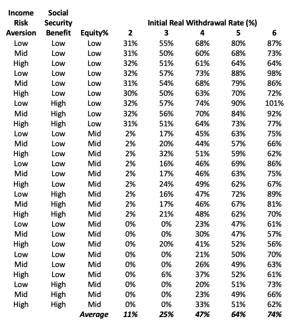
The table below shows the optimal equity allocations for a variety of scenarios.
Optimal PLIB equity allocations across household attributes, real withdrawal rates
There are two notable relationships given the optimal equity allocations in the table above. The optimal equity allocation for the PLIB increases for higher initial withdrawal rates. The effect is relatively monotonic and is due to the fact portfolios with higher equity allocations have higher expected returns and therefore create a higher probability of achieving a more aggressive equity target. If we assume the retiree household is using a 4% real withdrawal rate, which is approximately optimal, the average equity allocation would be approximately 50%.
There is a clear negative relation between the equity allocation for the non-annuity portfolio and the optimal PLIB allocation. In other words, the PLIB allocation decreases (increases) as the portfolio equity allocation increases (decreases). This is counter to optimal equity allocations for GLWB portfolios, where the most aggressive portfolio would generally be optimal given the put option nature of the income.
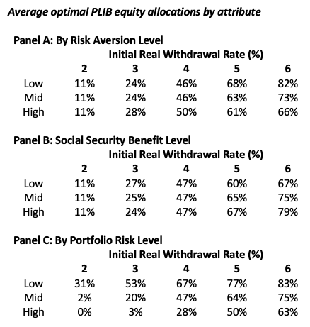
Those two effects are demonstrated in the following exhibit, which includes the average optimal equity allocations for the low, mid, and high values for each of the withdrawal rates considered.
Average optimal PLIB equity allocations by attribute
Again, the average equity risk levels vary by initial real withdrawal rate; high initial real withdrawal rates correspond to higher average equity levels. There are only minor differences in equity allocations across the risk aversion and Social Security benefit levels. There is a variation depending on the equity level of the regular portfolio (i.e., non-PLIB assets). This suggests the optimal equity allocation within a PLIB should be adjusted depending on not only the overall situation of the retiree (i.e., funded status) but on how the non-PLIB monies are invested.
Conclusions
Unlike GLWBs, which generally have restrictions on portfolio allocations, PLIBs allow for significantly more customization. In the future, PLIBs are likely to overlay a variety of portfolio structures, including variable annuities (VAs), registered index-linked annuities (RILAs), fixed indexed annuities (FIAs), as well as regular portfolios (e.g., as a contingent deferred annuities).
The ability to personalize the risk level will be valuable for those who purchase PLIBs. Those structures that allow for a wider range of risk exposures, especially riskier allocations (which may not be possible in a FIA) will better help advisors create more optimal strategies.
David Blanchett, PhD, CFA, CFP®, is managing director and head of retirement research at PGIM. PGIM is the global investment management business of Prudential Financial, Inc. He is also an adjunct professor of wealth management at The American College of Financial Services and a research fellow for the Retirement Income Institute.
Read more articles by David Blanchett