Why Volatility is the Wrong Measure of Investment Risk

Risk defined

There are a variety of definitions of investment risk, but the most appropriate one for the advisory profession is: “the chance that the investment strategy will not allow the investor to fulfil their aspirations and meet their obligations in life.” By this definition, there are many factors beyond volatility that will affect the client’s financial trajectory and outcomes.

Let’s start with the fact that risk is a one-sided concept, associated with the likelihood of negative outcomes, while volatility is a two-sided measure, treating good and bad outcomes equally. Most investors have an asymmetric view of variability, with more aversion to losses than attraction to gains. Volatility can provide estimates of the likelihood of negative outcomes, but it is more appropriate as a measure of variability than risk. Volatility doesn’t provide the client with an intuitive and practical understanding of that variability or its effects relative to their objectives.

Finally, high volatility includes the possibility of large positive outcomes that can outweigh the negatives.

Risk factors beyond volatility

Low volatility is typically associated with lower returns, which can increase the risk that a portfolio won’t generate sufficient capital growth or income to meet the client’s long-term needs. Many people approaching retirement will increase the fixed income portion of their holdings to reduce volatility, thinking they are also lowering their shortfall risk. However, in today’s low-yield environment, this could increase their shortfall. Because investors typically demand higher returns from higher volatility assets, a higher volatility position may be less likely to fall in value over longer time periods and less likely to fall short of investment targets.

A portfolio with historically low volatility may have hidden exposures to unexpected tail events caused by structural factors; for example, a popular investment style may be prone to sharp declines if many similar investors exit at the same time (also known as overcrowding).

Correlations increase in times of stress. A “low-volatility” fund can have a high-beta exposure to the market. Adding asset classes with high historical volatility can reduce risk if they are negatively correlated to the portfolio, mitigating the risk that all holdings will decline at the same time.

Finally, volatility measures don't uncover the risks inherent in concentrated stock positions. Two portfolios may have the same volatility, but one may be considerably riskier if, for example, it contains higher exposure to individual stocks.

Volatility doesn’t mean what people intuitively believe

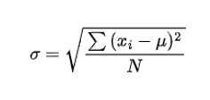
Your clients probably believe that an investment will move more/less than the standard deviation 50% of the time. But volatility is the square root of average squared deviation relative to the mean, defined by the formula:

Most people find this hard to conceive, and often misinterpret it as another common statistic, known as the mean absolute deviation (MAD), defined by the formula:

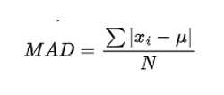Standard deviation is easier to work with mathematically, but mean absolute deviation is much easier to understand. When Karl Pearson first coined the term “standard deviation” in 1893, he used it as a simplification for the more descriptive “root mean squared error.” Standard deviation has become so popular that it’s impossible to change, but the choice of words has, to a large extent, contributed to the common misconception of what it means.

As a result, many clients might infer that two investments with the same standard deviation are equally risky. This is not the case, as demonstrated by the following simple mathematical example. Let’s consider three sequences of 10,000 numbers:

1. Random sample from a normal distribution with mean 0 and standard deviation 1
2. Alternating values 1 and –1: [1, -1, 1, -1, 1, -1, ....]
3. Constant small and positive values, with one large outlier: [0.01, 0.01, 0.01, ...., -100]

These sequences clearly have radically divergent behavior, as can be seen in the diagram.

Fig 1: sample sequences chart

But their statistical properties have some interesting similarities, including an identical standard deviation:

Fig 2: sample sequences statistics

Their mean and standard deviations are the same, but the mean absolute deviations (MADs) are very different. Furthermore, standard deviation doesn’t tell you anything about the nature of the distribution. Two data sets with the same standard deviation can have widely differing distributions, and a data set with relatively low standard deviation may have a small number of extreme values.

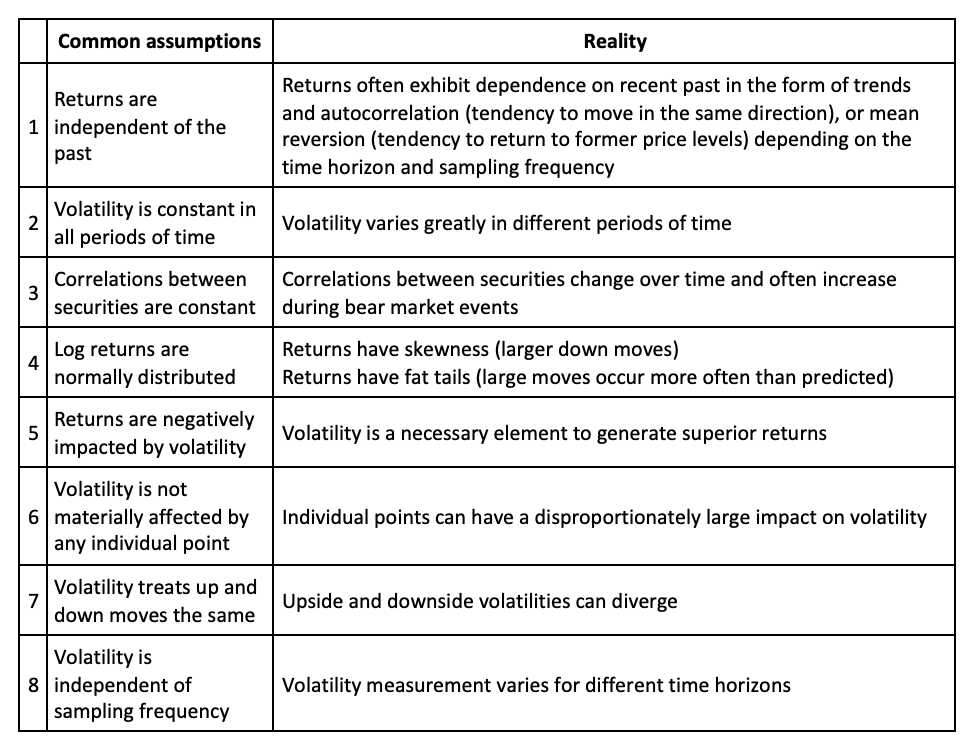
Assumptions versus reality

Below are several commonly held assumptions that have been adopted for convenience of financial analysis. This list provides some important guidance for how one might develop a more realistic approach to analyzing and measuring risk.

To show the difference between returns implied by standard deviation measurements and real-world results, I used SPY daily returns from 1/1/2007 to 10/31/2021. The chart below shows that most of the time, for small- and medium-sized moves, the returns track a normal distribution very well. But the largest moves (up or down) are much larger than those predicted by a normal distribution. Also, the size of these extreme moves is relatively larger for short sampling intervals.

In other words, extreme daily moves are proportionately much larger than monthly moves after adjusting for the sampling period. This suggests a degree of mean-reverting behavior not captured by traditional volatility statistics.

Fig 3: Q-Q plot of actual quantiles vs theoretical quantiles – 1D, 10D, 20D sampling

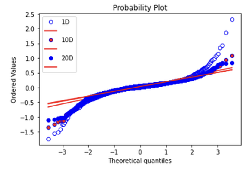
The type of scatter plot above is commonly used in statistics to compare two distributions and their quantiles against one another. Here we compare the observed market (S&P 500) returns to theoretical market returns from a standard normal distribution sampled at one-, 10- and 20-day intervals. Volatility would be a good measure of risk if actual returns were normally distributed, because we could use the two-sigma (95% probability) band to set expectations with clients and avoid surprises. If returns were in fact normally distributed, we would expect the scatter plot to form a straight line. However, as we can observe, the actual returns distribution deviates significantly from the standard normal distribution once we go beyond the two-sigma range (+/- 2 quantiles) and this deviation is higher at higher frequencies, which can lead to unexpected losses.

The implication of this analysis for advisors is that there is a big difference between what is expected and what is observed. Using the 95% probability or two-sigma bands to set expectations around performance may be setting clients up for a big surprise that could result in a bad experience, failure to stick to the plan and lawsuits. On the other hand, advisors with a deeper understanding of risk can be transparent with clients to better understand their emotional biases, proactively engage in conversations with clients to plan around big losses and set proper expectations to avoid costly mistakes. Additionally, advisors who take the unconventional approach to look beyond the two-sigma range for risk analysis will also differentiate themselves in a highly competitive profession.

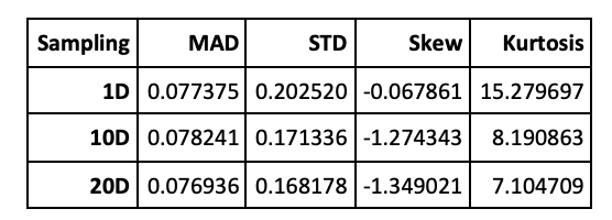
This graph is summarized mathematically in the table below. For shorter sampling periods, the standard deviation (annualized) is much higher, skew is smaller (more balanced between up and down moves) and the kurtosis is much larger (up and down moves are larger).

It illustrates a few real-world portfolio issues that traditional measures of risk don’t capture:

• Large short-term moves tend to mean revert over longer timescales.
• Asymmetry of returns is only visible over longer sampling intervals.
• Heavy tails (while present at all frequencies) are more pronounced over short timescales. The divergence from normal distributions is evident (for a normal distribution, skew = 0 and kurtosis = 3).

Fig 4: SPY statistical metrics as a function of sampling interval

Variability of volatility over time

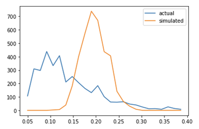
Finally, below are two charts that further highlight the contrast between reality and a constant volatility model. The volatility over this period is approximately 0.2, which conforms to a long-term statistic. However, if we take a rolling 30-day sample using volatility=0.2 and compare that to market history, we see that most of the time the actual volatility was much less than 20, with occasional spikes during periods of great market stress.

The range of daily scenarios leading from a constant volatility number are not at all representative of what an investor will experience.

Fig 5: Time series of rolling 30-day volatility, actual vs theoretical

Fig 6: Frequency distribution of rolling 30-day volatility, actual vs theoretical

Alternative risk metrics to overcome the limitations of volatility

Using volatility as the sole risk measure inevitably steers an investor towards strategies that preserve a fixed monetary value But for most investors, the absolute value is not as important as the value relative to their future needs. People approaching retirement don’t need a fixed asset-value target but want to ensure that they will be able to maintain a certain income and lifestyle in the presence of a variety of changing factors: inflation, changing market valuations, asset returns and withdrawal rates.

There are a few alternative risk metrics that are better aligned with a client’s investment objectives. They can be used to evaluate a portfolio through different lenses and come up with a more reliable and comprehensive view of its inherent risks:

1. Tail risk – the chance that a seemingly low-risk product could experience unexpectedly large losses;
2. Lack-of-diversification risk – which can be mitigated by introducing assets that have lower correlation to the investments in the portfolio;
3. Shortfall risk – possibility of investments will not meet the client’s target objectives, due to a concentration of assets that have historically produced lower returns; and
4. Concentrated-stock risk – sizable holdings in a small number of stocks that could increase idiosyncratic risk tied to those companies' performance.

Advisors can help their clients mitigate the risks they face by addressing more than just the volatility of their investment portfolios – and help them understand that volatility is at best an inaccurate measure of the risks they're taking. At worst, it is a misleading guide to the most practical way for them to invest for their retirement future. An accurate depiction of risk for clients requires a three- or four-dimensional model covering all aspects of the dangers lurking unseen in retirement portfolios.

Akhil Lodha is the CEO at StratiFi, a financial technology company empowering investment advisors to enlighten clients about risk to differentiate themselves, get better insights to build robust portfolios, and monitor accounts automatically to reduce business risk. Its online platform gives investment advisors access to sophisticated risk management technology normally only accessible by the largest institutions.

Read more articles by Akhil Lodha