The following is excerpted from Chapter 10 in Wade Pfau’s new book, Retirement Planning Guidebook: Navigating the Important Decisions for Retirement Success. It is available at Amazon, Barnes & Noble, Target, and other leading retailers.
Here is an example that quantifies how strategic tax planning and delayed Social Security claiming can increase portfolio longevity in retirement. I have created an example for a 60-year-old single individual who has just retired in 2021. She has $2 million of investment assets, divided between $400,000 in a taxable account, $1.3 million in a traditional IRA, and $300,000 in a Roth IRA. The cost basis for her taxable assets is also $400,000. Her goal is to spend $95,000 a year in retirement net of any federal income taxes and she lives in a state that does not tax income. For Social Security, her primary insurance amount is $30,000 if she claims at her full retirement age of 67. She will get $21,000 if she claims at 62 and $37,200 if she claims at 70.
This example does not incorporate asset location issues and long-term capital gains management, as I simplify investment returns to be 2 percent annually with no inflation. This implies that investments are held in bonds and provide 2 percent taxable interest payments annually without potential for capital gains or losses. While investment returns are simplified, the full tax code has been built into the example. Taxes for 2021 to 2025 are based on present law, and the 2017 tax code (with inflation adjustments through 2021) is used for 2026 and later.
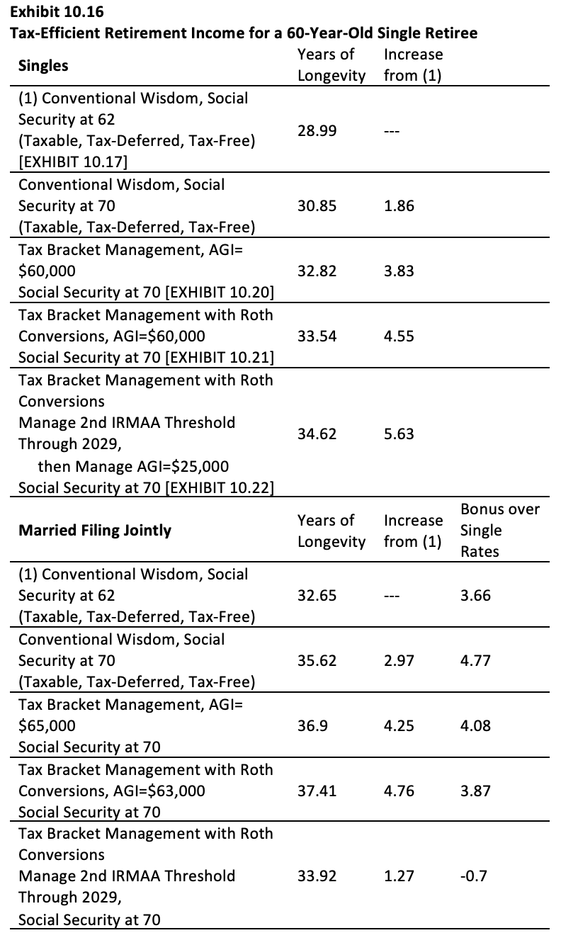
Exhibit 10.16 summarizes the results for this example. It shows five different strategies for this individual. The first is to claim Social Security at age 62 and to follow the conventional wisdom for spending down assets: take any RMDs, then spend the taxable portfolio, then the tax-deferred portfolio, and then the tax-exempt portfolio. This strategy supports 28.99 years of retirement spending, and the details are provided in Exhibit 10.17. It is the baseline. When the portfolio covers a fraction of the year, that represents the percentage of the overall spending goal that can be funded in the year.
Next, to show the value of delaying Social Security, if this retiree claims Social Security at 70 and uses the same conventional wisdom spend-down strategy, portfolio longevity increases by 1.86 years to 30.85 years. The remaining strategies in the exhibit also use Social Security claiming at 70. The next strategy is to use tax bracket management at a pre-determined level of AGI without using Roth conversions. I test various AGI levels to manage and find that an AGI target of $60,000 provides the most benefit for this example, with portfolio longevity of 32.82 years (see Exhibit 10.20). If we follow the same strategy and include strategic Roth conversions as well, portfolio longevity increases to 33.54 years (see Exhibit 10.21). Coincidentally, an AGI target of $60,000 also creates the greatest portfolio longevity with Roth conversions. Finally, I provide an example of front-loading taxes to a higher level in the early retirement years and then targeting a lower AGI level for later in retirement. After several different permutations, I find that managing AGI to $111,000 until age 70, which is the threshold just before a second layer of IRMAA-related Medicare premium increases kick in for earnings starting at 63, and then switching to manage an AGI of $25,000 for age 70 and later (when Social Security starts) can increase portfolio longevity by more than another year to 34.62 years (see Exhibit 10.22). This is 5.63 years longer than following convention wisdom on spenddown strategies and claiming Social Security early. After raising the claiming age to 70, this more tax-efficient strategy still adds 3.77 years of portfolio longevity to the convention wisdom tax strategy. The topics described in this chapter can add significantly to the longevity of retirement distributions.
As a further note, this exhibit also shows the five corresponding strategies assuming that everything is the same except that the discussion is about a married couple instead of a single person. The point for including results for the couple is to demonstrate how much impact the differing tax brackets between singles and couples can have on retirement sustainability. For the different strategies, applying tax brackets for married filing jointly could extend portfolio longevity by more than 3.66 years. This does speak to the planning idea mentioned about how those who are married filing jointly may seek more balance by frontloading taxes in anticipation of an inevitable point when the surviving spouse will face the tax brackets for singles. We can also note that the strategy for managing the second IRMAA threshold for couples ($222,000) is too aggressive and results in worse outcomes. It forces too much taxes to be paid early on, such that tax capacity is wasted later in retirement.
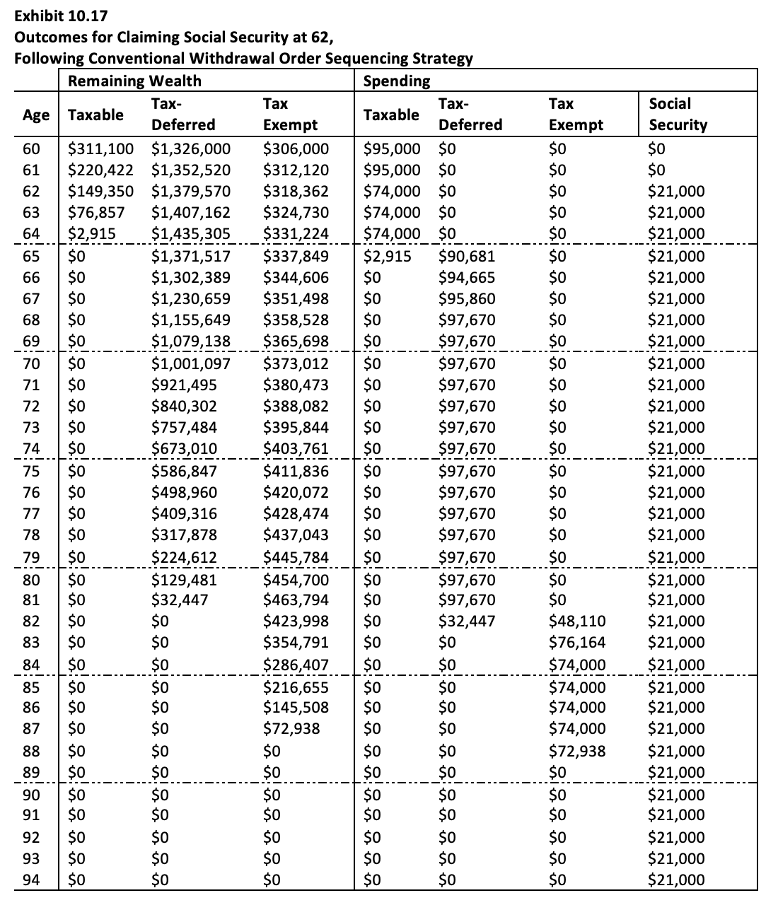
Moving now to the specific lifetime patterns for different strategies, Exhibit 10.17 provides the results for claiming Social Security at age 62 and following the specific distribution strategy of spending taxable assets first, then tax-deferred assets, and then tax-exempt assets. In this case, she can meet her full spending goals for 28.99 years until just before her 89th birthday. At this point her investment assets deplete and she only has a $21,000 Social Security benefit to cover the rest of her life. I show the details of this strategy to contrast it with more efficient spending strategies.
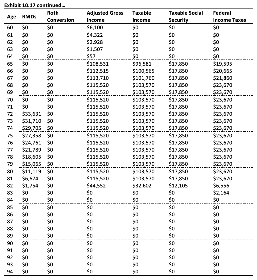
In Exhibit 10.17, we can identify some of the inefficiencies with the standard withdrawal recommendations. First, by only spending from the taxable portfolio at the start, she wastes space in her tax brackets to trigger taxes when tax rates are low. Her adjusted gross income in the early retirement years consists only of the 2 percent interest payments being generated by her remaining taxable assets each year. Her income does not even rise to the level of the standard deduction until age 65, when her taxable assets deplete, and she switches to spending from the tax-deferred account. Though she does not pay taxes during the first 5 years of retirement, she is heading toward a bigger tax bill later that will have a profound effect on her portfolio longevity.
From ages 65 to 81 her adjusted gross income is more than $100,000 because she spends only from the tax-deferred account and Social Security benefits. This inefficiency is leading her to have tax payments on 85 percent of her Social Security benefits between the ages of 65 and 82. In addition, from ages 66 to 81 her Medicare MAGI (I assume no tax-exempt bonds so this MAGI matches the AGI) exceeds the second Medicare threshold ($111,000), which causes her Medicare premiums to increase by $2,164 per year from ages 68 to 84. Remember, Medicare premiums have a two-year lag related to income. I include these IRMAA increases as part of her taxes. Her annual tax bill between ages 68 and 82 is $23,670, which represents an effective tax rate of 24.9 percent of her $95,000 pre-tax spending goal. As discussed at the outset of the chapter, this is a meaningful way to describe the effective tax rate in retirement.
Later in retirement, after she depletes the tax-deferred account, spending is sourced to the Roth IRA and Social Security. Her taxes eventually fall back to $0 as her adjusted gross income is $0 starting at age 83. That year she just has one more IRMAA adjustment to pay. Roth distributions do not create any taxable income, and her Social Security benefits are not taxable at this stage. While taxes are $0 as of age 84, the damage has already been done and there is 0 percent tax rate capacity being wasted by not having income to cover the standard deduction.
One other harmful possibility that was not an issue with this example is that required minimum distributions were never binding in terms of forcing a higher distribution from the tax-deferred account than the retiree otherwise wanted, but this could also be an issue for those whose IRA balances are too high relative to their spending goals. This distribution strategy simply missed opportunities to pay taxes at lower rates and ended up paying too much tax at higher rates.
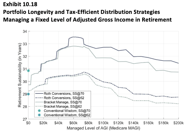
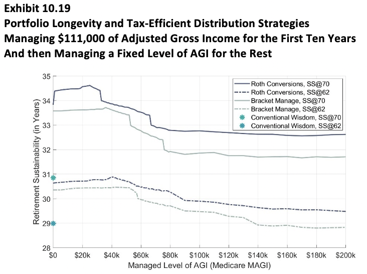
As we shift to more efficient strategies, Exhibits 10.18 and 10.19 helps us identify how the AGI target choice impacts portfolio longevity. These exhibits become the source of the strategies we consider in greater detail in subsequent exhibits. The strategy we just described is represented as “Conventional Wisdom, SS@62” in these two exhibits. We can contrast the conventional wisdom approach to tax bracket management either as the source of retirement spending (Bracket Manage) or to conduct strategic Roth conversions (Roth Conversions). For these strategies, the level of AGI managed impacts portfolio sustainability and the charts can be used to find the income level linking to the longest sustainability.
In Exhibit 10.18, we consider a variety of fixed adjusted gross income levels to manage and study portfolio longevity as we vary income targets. Generally, allowing Roth conversions can support greater portfolio longevity. The exhibit shows that for this example, using Roth conversions and managing an adjusted gross income of $60,000 per year allows for the greatest portfolio longevity. It is the sweet spot to provide the best balance for lifetime taxes. Lower AGI levels will not be able to get enough moved to the Roth account and can lead to too much later taxes. Higher levels mean moving assets to the Roth account too quickly such that some of the lower tax bracket space is eventually wasted by a lack of taxable income.
Exhibit 10.19 takes matters a step further to show how managing to the $111,000 AGI level for the years before Social Security begins and then managing to a lower subsequent level may support even better outcomes. This front-loading of taxes reduces the impact of the Social Security torpedo later in retirement, as by that time managing an AGI of $25,000 can support the most long-term sustainability. Using the optimal outcomes from these two exhibits give us the sources for additional examples to explain how tax bracket management can improve portfolio sustainability.
(skipping ahead…)
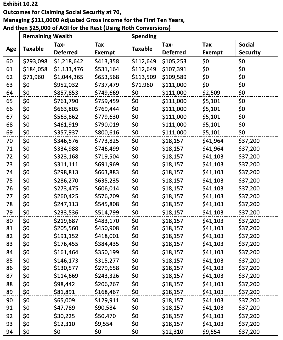
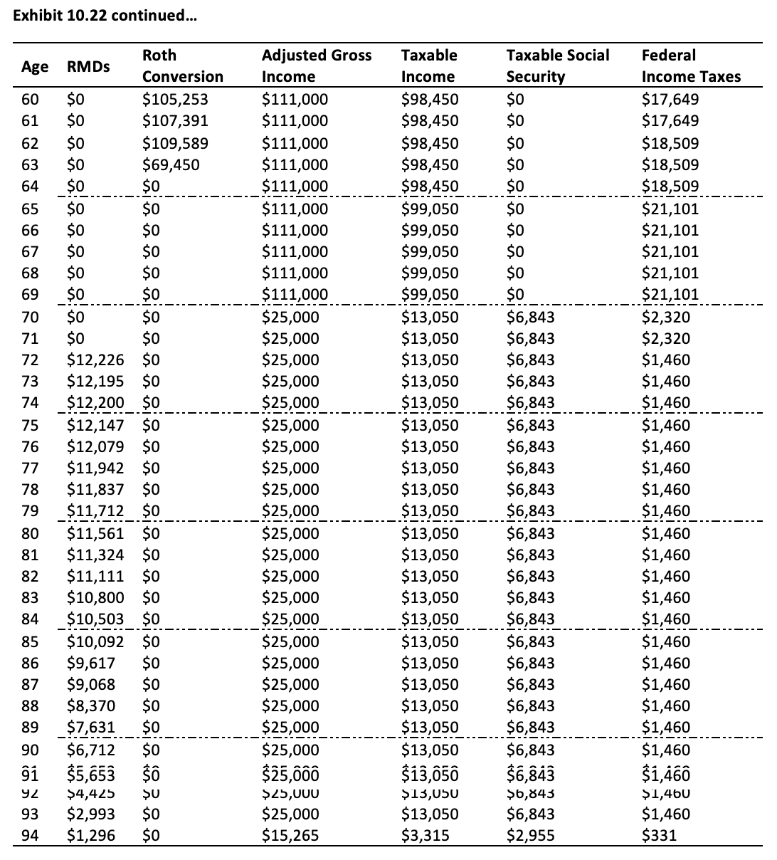
As a final example, Exhibit 10.22 provides a case in which taxes are even more strongly front-loaded into the early retirement years before Social Security begins. This helps to better manage the Social Security tax torpedo. Even though tax bills are higher in the early retirement years, the strategy can increase portfolio longevity by more than a full year relative to the previous strategy. This strategy allows the retirement spending goal to be met for 34.62 years.
In this case, Roth conversions are used to manage a $111,000 AGI level for the first ten years of retirement before Social Security begins. As I am assuming there is no tax-exempt interest from municipal bonds to be counted, the AGI matches the MAGI used to calculate IRMAA-related premium increases for Medicare. This AGI target is right at the level that accepts one hike in Medicare premiums but just avoids the second hike. In practice, one must be especially cautious about managing income around one of the Medicare brackets, because going over by just $1 will trigger a substantial additional premium hike.
This strategy allows for larger Roth conversions in the early years of retirement until the taxable portfolio depletes at age 63. Roth conversions exceed $100,000 for three years but are limited in the fourth year by the small remaining balance for taxable assets. The spending is then sourced to a combination of tax-deferred and Roth distributions to continue managing the same AGI level through age 69.
At age 70, Social Security begins and a new AGI target of $25,000 is used for the remainder of retirement. Though the tax bill reaches $21,101 for ages 65 to 69, it is only $2,320 at age 70 and 71 and then never exceeds $1,460 for the remainder of retirement. Required Minimum Distributions are never binding to force more from the IRA than is desired for spending and tax-efficiency purposes. This $1,460 tax number provides an effective tax rate of 1.5 percent of the retirement spending goal for ages 72 and later, which may seem shocking for someone who began their retirement with $2 million of investment assets and is managing $95,000 of pre-tax spending. The reason this strategy is so effective is because it worked to further reduce the Social Security tax torpedo, as only 18.4 percent of Social Security benefits are counted as taxable income throughout retirement. Portfolio assets last for 34.62 years until the retiree is almost 95 years old. This is an increase of 5.63 years over the baseline, showing the real value that can be obtained for retirement plans by combining a delay in Social Security with an aggressive Roth conversion strategy in the early retirement years.
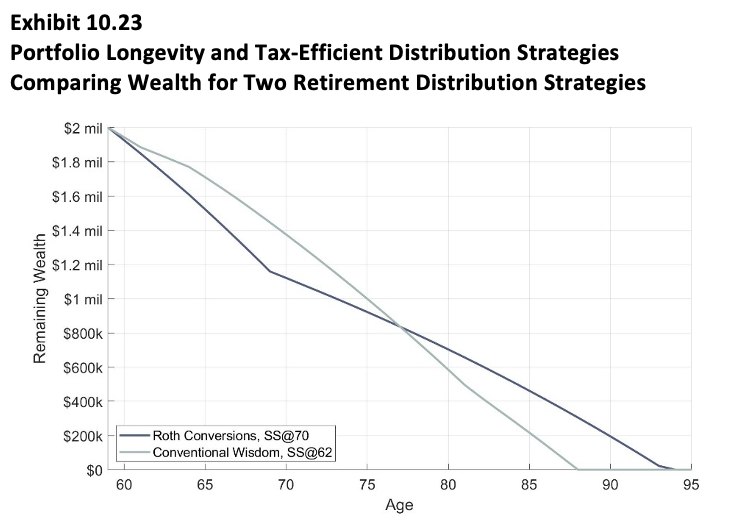
I conclude this example with Exhibit 10.23, which could serve as the guiding emblem for this book. It tracks remaining wealth in retirement for the longest surviving strategy from Exhibit 10.22 against the baseline strategy from Exhibit 10.17. This image shows the tradeoff between short-term costs and long-term benefits for the two strategies. We described how delaying Social Security to 70 and aggressively making Roth conversions allows for retirement assets to last 5.63 years longer while meeting the same pre-tax spending goal, as compared to a strategy in which Social Security is claimed at 62 and assets are spent in order from taxable, tax-deferred, and then tax-exempt accounts. The exhibit shows how obtaining these long-term benefits requires short-term sacrifice, as the tax-efficient strategy will lag with its remaining wealth for the first 17 years of retirement. For the largest early gap, the baseline strategy supports $286,283 more at age 69, as the long-term winning strategy has been spending investment assets faster to cover missing Social Security benefits and higher tax bills. After age 70, the trend reverses. The crossover happens at age 77 when there is about $840,000 left with both strategies. The more efficient long-term strategy provides the largest advantage at age 88 with $323,057 left when the baseline strategy runs out of assets.
For someone who is more focused on the short-term, the baseline strategy could have appeal. Legacy values will be larger if death happens before age 77. But age 77 is before life expectancy so that there is more than a 50 percent chance that life will continue to an age where the efficient strategy performs better. As well, in both cases legacies will be relatively large with an early death. If death happens at 69, the baseline strategy provides $1.44 million of legacy. But the $1.16 million remaining with the efficient strategy is still quite large. Retirees might focus more on the legacies with a longer retirement, where dollar values are less, and each dollar of legacy can have a bigger impact. For instance, with death at age 88, one strategy provides $323,057 of legacy while the other provides $0. For those living beyond 88, reverse legacies may come into play as retirees outlive their assets and come to rely on the support from others. A case can be made for either strategy, though I would suggest serious consideration should go to the strategy creating the most long-term benefit. It is important to consider these trade-offs when thinking about the right approach.
The Retirement Planning Guidebook is designed to help readers navigate the key financial and non-financial decisions for a successful retirement. The book includes detailed action plans for decision making that can assist advisors and their clients. It is available at Amazon, Barnes & Noble, Target, and other leading retailers.
Wade D. Pfau, Ph.D., CFA, is the curriculum director of the Retirement Income Certified Professional program at The American College in King of Prussia, PA. He is also a principal and director at McLean Asset Management and RetirementResearcher.com.
 The following is excerpted from Chapter 10 in Wade Pfau’s new book, Retirement Planning Guidebook: Navigating the Important Decisions for Retirement Success. It is available at Amazon, Barnes & Noble, Target, and other leading retailers.