Annuities can reduce the risk of running out of money in retirement, but they protect against this risk in different ways. I’ll compare retirement outcomes for single-premium immediate annuities (SPIAs) to guaranteed lifetime withdrawal benefits (GLWBs) to understand the key product differences.
As background income annuities provide a lifetime income in exchange for an up-front premium and may be either SPIAs or deferred income annuities (DIAs). Another approach to providing lifetime income is GLWBs offered as an optional rider to variable annuities (VAs) and fixed index annuities (FIAs). These riders allow withdrawals to continue for life even if annuity account values are depleted.
Income annuities
Income annuities are the simplest product – you pay a fix sum up front and receive a predetermined payment per month for life. With SPIAs, income payments begin immediately, while with DIAs, the commencement of income is delayed. For example, a 65-year-old might purchase a DIA with payments commencing at 85 in order to provide longevity protection or funds for long-term care. The government even sanctions this type of DIA for tax-deferred accounts as a qualified longevity annuity contract (QLAC) so that required minimum distributions (RMDs) can be delayed. SPIAs and DIAs can be structured with either level payments or payments that step-up by a given percentage each year. A few companies formerly offered SPIAs where payments increased each year based on actual inflation – an ideal add-on to Social Security – but this product is no longer offered due to lack of demand.
VAs and FIAs with GLWBs
While income annuities have been available in various forms for thousands of years, GLWBs only have a 20-year history. First they were offered as an optional rider on VAs and then later on FIAs as FIAs became more popular. With GLWBs, there is a maximum allowable initial withdrawal percentage that increases with age – 5% of the VA or FIA account value at age 65 is typical. A shadow account, or benefit base, is set up when the first withdrawal is taken and this benefit base will never decrease, but can increase (ratchet-up) if the account value grows to be greater than the benefit base. The allowable withdrawal percentage, set at the initial withdrawal, is applied to the benefit base. Hence, allowable withdrawals can increase, but never decrease below the initial allowable level. The allowable withdrawal level then continues for life, even if the underlying account value is depleted. With GLWBs, the annuity owner can surrender the contract, giving up withdrawals guarantees, and thus have access to the full remaining account value. For SPIAs and DIAs there is no account value, although some offer an option for payments for early deaths.
Sales history
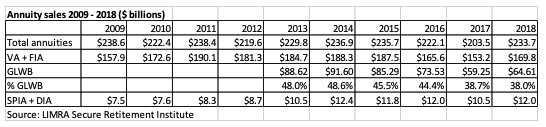
The chart below, provided by the LIMRA Secure Retirement Institute, shows a 10-year sales history from 2009-2018 for VAs, FIAs, and income annuities, plus more recent history for both VA and FIA sales where a GLWB rider was purchased.

Total annuity sales for 2018 were quite close to peak sales levels achieved at various points during the 10-year history. VA sales decreased since 2015, but for 2018 in particular, sales of FIAs and other fixed-rate annuity products received a boost from higher interest rates. The decreased percentage of GLWB sales since 2016 is surprising and there is no clear explanation. There may have been some pulling back in the past few years due to uncertainty over the imposition of rules about sales practices. SPIA and the smaller amount of DIA sales have increased somewhat over the 10-year history, but still remain at modest levels – less than one-fifth of GLWB sales. It seems that individuals have a strong desire to maintain control and access to their savings, which they retain with VAs and FIAs, but lose with income annuities. Another explanation is that VAs and FIAs are more aggressively marketed than SPIAs and DIAs.
Comparing SPIAs to GLWBs
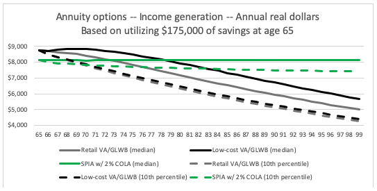
The chart below compares income projections for one particular SPIA and two versions of a VA with a GLWB. The results are shown in real dollars with inflation removed to demonstrate what happens to purchasing power. I show median results and also the 10% percentile as a downside measure.
The SPIA pricing is as of early January 2020 from annuity research firm CANNEX, and the particular product structure is one where the income payments increase by 2% each year – known as a 2% COLA. I used Monte Carlo projections, assuming 2% average inflation with a 1.3% annual standard deviation, approximately the amount of variability we have seen over the past 40 years.
Because the SPIA COLA is 2% and assumed inflation is 2%, the median real income projection is flat at just over $8,000. The 10th percentile declines from this level, reflecting Monte Carlo outcomes that are worse than average inflation. Variability in real income is only due to variability in inflation; there is no impact from other economic variables.
For GLWBs, I provide two examples, one based on a typical retail product with annual charges totaling 3.5% and a low-cost or institutional version with total charges of 1.5%. For the Monte Carlo projections, I assume a 60/40 stock/bond mix for the VA accounts with a mean real return of 3.4% (lower than historical averages) and standard deviation of 12.3% (roughly equal to the long-term historical average). The initial allowable withdrawal rate at 65 is 5% for both GLWBs.
Results for the GLWB show real income that is expected to decline, and the difference between median and 10th percentile results indicates how variable the income can be. This portrayal of what is likely to happen to real spending power is at odds with how GLWBs are marketed, which focuses on nominal income never decreasing and likely to ratchet up. This stark difference was brought home to me by Bill Sharpe’s RISMAT text, which I reviewed in this Advisor Perspectives article.
In contrast to the SPIA, the difference between median and 10th percentile results are impacted by both variability in inflation and investment performance. The median results for the two GLWBs are quite different, but the 10th percentile results are almost the same. This is because the 10th percentile results for both cases have the same initial assumed withdrawal and 10th percentile nominal withdrawals stay close to this level without a significant ratcheting up from investment performance.
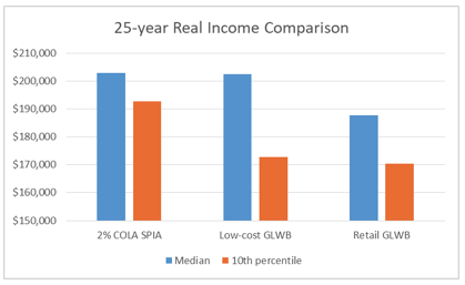
The chart below provides total real income projections for equal purchase amounts of these three annuity options over 25 years, the approximate expected lifetime for a 65-year-old female annuity purchaser.
For median outcomes, the 2% COLA SPIA and low-cost GLWB are close to a tie, but the COLA SPIA does better on downside risk as represented by the 10th percentile results. The retail GLWB does worse in terms of the median, but has about the same downside as the low-cost GLWB, as noted earlier.
Accessible wealth
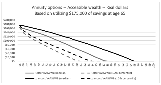
It is advantageous for individuals to maintain control and access to savings, and the chart below compares the two versions of GLWBs. For the SPIA example, there would be no accessible wealth.
The retail GLWB starts below $175,000 because I assume surrender charges of 7% grading down over seven years, but no surrender charges on the low-cost product. The age at which the account balance hits zero is when the lifetime withdrawal guarantee kicks in. Until that age, one is simply withdrawing their annuity account balance. For example, with the low-cost product assuming a median result, one would need to live until at least 95 for the lifetime withdrawal guarantee to kick in.
Because the annual charges for both types of GLWBs are significantly higher than one would expect to pay for low-cost mutual funds of ETFs, the account balances go to zero earlier than would be the case taking the same year-by-year withdrawals from regular investment accounts. However, regular investment accounts would not provide continuing withdrawals after accounts were depleted.
Tradeoffs
There no one clear best answer in helping clients choose amongst annuity products. The key differences between income annuities and GLWBs involve downside protection for income (favoring income annuities) versus access to and control of funds (favoring GLWBs). For GLWBs, lower charges clearly lead to better product performance – particularly for median results and upside. Retail (i.e., expensive) pricing of GLWBs currently dominates in the marketplace with low-cost GLWBs sold to a small minority of direct purchasers who don’t buy from a broker or insurance agent. However, recent passage of the SECURE Act, part of which encourages company retirement plans to offer annuities, may change that balance. Plan sponsors will need to determine which types of annuities to offer and there will certainly be pressure to keep expense charges down if GLWBs are offered.
Broader context
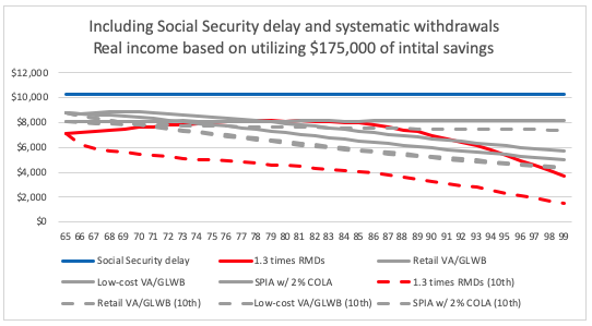
In the chart below, I show the median and 10th percentile income projections that we have looked at already in gray (for the SPIA and two versions of a GLWB), and also show two other options for utilizing savings to generate retirement income – Social Security delay, and using systematic withdrawals that don’t involve an annuity purchase.
Social Security delay is akin to a SPIA purchase. For the particular example of utilizing $175,000 of savings, we can do some reverse engineering and calculate that an individual who would collect a monthly Social Security benefit of $2,059 at 65, could instead wait until 70 and begin collecting $2,917, a 42% increase. They could still retire at 65 and use $175,000 of savings (60 months times $2,917) to set up a bridge fund to begin paying themselves this higher amount at age 65, and then transition to Social Security at age 70. (Because Social Security benefits adjust each year for inflation, these numbers are all in real dollars.) In effect they would be using $175,000 of savings to purchase additional income of $858 per month ($2,917 - $2,059), or $10,296 per year.
When we put that $10,296 on the real income chart, we see that it is a level amount because it adjusts each year for inflation. I don’t have a separate 10th percentile line because it is not subject to inflation risk or investment risk. There may be some risk due to future changes in government entitlement policy; it will depend on particular changes that are only speculation at this time. Overall, we see from the chart that there is a compelling case for Social Security delay versus income annuities or GLWB options. However, these annuity products can provide additional lifetime income if desired.
There are a wide variety of methods for taking systematic withdrawals from savings. The particular approach shown in the chart involves a more aggressive approach to taking RMDs – taking 1.3 times the specified RMD amount. I chose this approach because it produced real withdrawals at age 90 (life expectancy) about equal to the initial level of withdrawals and produced total real withdrawals up to life expectancy that were similar to totals from the annuity approaches. I assumed a 60/40 stock/bond mix as I did for the GLWBs.
The 10th percentile projection on the chart shows that there is significant downside with this systematic withdrawal approach. We would see a similar result with other systematic withdrawal approaches with a similar stock/bond mix. However, if we did an accessible wealth analysis, we’d find systematic withdrawals beating the GLWBs, which have the drag of annual charges of 1.5% to 3.5%, and we’d expect much smaller charges for pure investment portfolios.
Final word
For building sustainable lifetime income, my view is that the first place to look is Social Security delay (and coordinated strategies for couples). If more lifetime income is desired, the next step should be examining income annuity and GLWB options, and being mindful of the tradeoffs involved to determine what works best for particular clients. I favor generating enough lifetime income to cover basic living expenses and leaving systematic withdrawals for discretionary spending where it’s feasible to adjust spending from year-to-year.
Joe Tomlinson is an actuary and financial planner, and his work mostly focuses on research related to retirement planning. He previously ran Tomlinson Financial Planning, LLC in Greenville, Maine, but now resides in West Yorkshire, England.
More ETF Topics >