Advisor Perspectives welcomes guest contributions. The views presented here do not necessarily represent those of Advisor Perspectives.
The seasonal effect, namely that equities do better from November through April, is well-known. This article provides a rigorous statistical test of the effect and a trading strategy that profits from it.
My long-term study supporting this observation can be found here. A related switching strategy model with cyclical and defensive ETFs is described here.
The seasonality of the S&P 500 is easily verified. The S&P 500 with dividends from 1960 onward returned on average 1.92% for the six-month periods May through October, the “bad-period.” For the other six months, the “good-period,” from November through April, the average return was 8.47%.
Visually observing is not an adequate way to assess effectiveness. It is more rigorous – but nonetheless quite easy – to statistically demonstrate that the six months from November to April are usually good-periods for equities. The null hypothesis H0 is the default position, namely that there is no difference between the average returns of the good-periods and bad-periods, the average return hereinafter referred to as the “H0-return”.
Quantifying stock market seasonality with likelihood ratios
In evidence-based medicine, likelihood ratios assess the reliability of a diagnostic test, leading to improved patient outcomes and refined drug regimens. In finance, likelihood ratios can quantify the reliability of a financial test as well. For example, one can check the dependability of a recession indicator, as described here.
In medicine, likelihood ratios estimate how much the probability that a patient has a particular disease changes from before a diagnostic test is given to after its result is known. One can use the same concept to determine the probability of stock market performance over a particular period in the year when the outcome of a relevant indicator’s test is positive or negative.
The time over which I tested this is from January 1960 to April 2019, consisting of 59 cyclical good-periods (condition positive) and 59 cyclical bad-periods (condition negative) for stocks, totaling 118 six-month periods, and showing an average return of 5.20% for all periods, the H0-return.
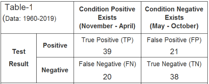
An indicator can be sending one of the following four messages, depending on the actual return for a period and its magnitude relative to the H0-return. For the condition positive the possibilities are:
- a correct call that the return for the good-period is greater than the H0-return (true positive, TP); or
- a false call (false positive, FP) when the return for the good-period is less than the H0-return.
For the condition negative the possibilities are:
- a valid negative call that the return for the bad-period is less than the H0-return (true negative, TN); or
- a wrong negative call (false negative, FN) when return for the bad-period is greater than the H0-return.
How often one of those conditions occurs over the observation period are the raw data for the analysis, shown in the Table-1 for my specific investigation.

There is a 65.0% probability that the good 6-month periods from November to April will produce higher returns than the H0-return of 5.20%, and a 65.5% probability that the bad 6-month periods from May to October will produce lower returns than the H0-return.
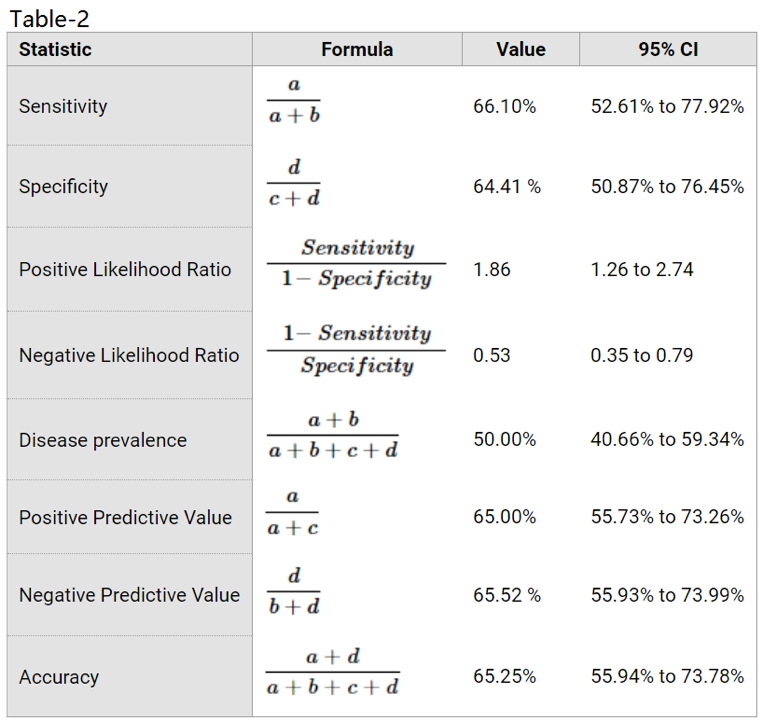
Here is a link to an on-line diagnostic test calculator, with the input being the data of Table-1 with a= TP, b= FN, c= FP, and d= TN. The output from the calculator, with 95% confidence intervals (CI), is listed in Table-2. Definitions of the various statistical terms are on the linked website.
The positive likelihood ratio is 1.86 with a 95% confidence interval of 1.26 to 2.74; a value greater than 1 produces a post-test probability which is higher than the pre-test probability (the ”disease prevalence” in the statistics below).
The positive predictive value in the statistics (another name for the positive post-test probability) is 65% with a 95% confidence interval of 55.7% to 73.3%, denoting statistical significance because the lower confidence interval of 55.7% is higher than the pre-test probability of 50.0%.
Profiting from stock market seasonality
Now that we have quantified the effect of seasonality on equities, we can design a reliable strategy to profit from it. We want to have more aggressive investments during the good-periods, and more defensive ones during the bad-periods.
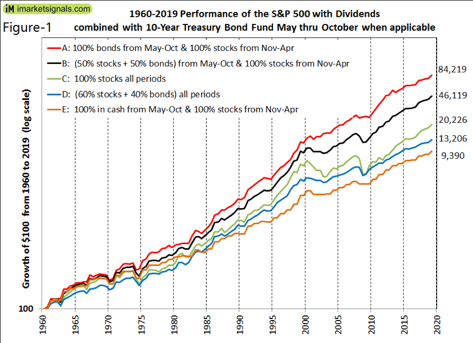
My strategy is to invest in the S&P 500 during the good-periods from November to April. For the bad-periods, May to October, there are numerous investment possibilities. I considered five alternatives to demonstrate the effect of seasonality. Models A, B, and E follow a seasonally variable allocation strategy, while C and D are fixed allocation models:
A. 100% bonds (10-Year Treasuries) during the bad period
B. 50% bonds and 50% stocks during the bad period
C. 100% stocks (buy-and-hold) all periods
D. 60% stocks and 40% bonds all periods
E. 100% cash without interest during the bad period
For the equity investment, I simulated daily prices for a hypothetical S&P 500 index fund by splicing the data from three sources: the SPDR S&P 500 ETF (SPY) from 1993 to 2019, the Vanguard 500 Index Fund (VFINX) from 1980 to 1993, and before that from 1960 to 1980 daily data of the S&P 500 with dividends taken from the Shiller CAPE data.
For the fixed income investment, I simulated daily prices for a hypothetical 10-year Treasury bond fund with data from three sources: from 1995 to 2019 the price of the iShares 7-10 Year Treasury Bond ETF (IEF), from 1962 to 1995 the 10-Year Treasury Rate from the U.S. Department of the Treasury, and before that the 10-Year Treasury yield from the Shiller CAPE data.
The performance over 59 years from May 1960 to April 2019 for the five alternative models is shown in Figure 1, with data plotted at six-month intervals. All trading was assumed to occur at the end of the last week of April and October.
Model A shows the highest performance: $100 would have grown to $84,219 equivalent to an annualized return of 12.1%, while Model C (buy-and-hold equity) would have produced only $20,226 for an annualized return of 9.4%.
The typical retirement savings strategy of holding 60% stocks and 40% bonds (Model D) is also one of the poor performers; $100 would have grown to $13,206 equivalent to an annualized return of only 8.6%.
For the more recent performance of the seasonal SPY-IEF switching strategy, from January 2000 to April 2019, see Figure-2 in the Appendix.
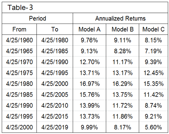
Annualized returns over consecutive 20-year periods for Models A, B, and C are listed in Table-3. It is evident that it would always have been more profitable, even during the period 1960-1983 of rising interest rates, to have some fixed income investment during the bad-periods from May thru October. Over any of the nine periods Model A always produced the highest return.
Conclusion
Based on the data since 1960, likelihood ratios confirm the seasonality of the stock market. The diagnostic test provides a 65% probability for the S&P 500 to perform better than average from November thru April, and a similar probability for the S&P 500 to perform worse than average from May thru October, indicating causation, namely that stock market returns increase or decrease due to seasonal effects.
Therefore, reducing equity allocation during the bad-periods of May thru October each year and replacing equity with fixed income during those months is expected to be a winning strategy over the longer term.
Georg Vrba is a professional engineer who has been a consulting engineer for many years. In his opinion, mathematical models provide better guidance to market direction than financial "experts". He has developed financial models for the stock market, the bond market, yield curve, gold, silver and recession prediction, which are updated weekly or monthly at http://imarketsignals.com/. Georg can be reached at [email protected].
Appendix
Profiting from stock market seasonality Jan-2000 to Apr-2019
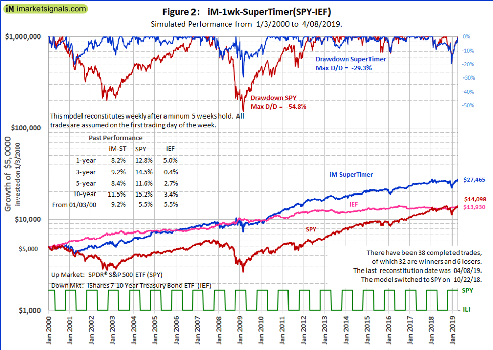
The performance of a seasonal switching strategy SPY-IEF since Jan-2000 is shown with the iM-1wk-SuperTimer in Figure-2.
The iMarketSignals’ weekly updated iM-SuperTimer defines up-market and down-market periods for stocks. It uses a combination of 15 unrelated market indicator models (including the seasonal model), all updated weekly.
For the seasonal switching strategy 14 of its component market timer models were turned off, only leaving the seasonal timer model on. Growth is plotted to a logarithmic scale, and the investment periods for stock fund SPY and bond fund IEF are depicted by the lower green graph in the figure.
Over the backtest period of more than 19 years a $5,000 initial investment would have grown to $27,465 by seasonally investing in SPY or IEF, for an annualized return of 9.2%. A $5,000 buy-and-hold investment in SPY or IEF would only have grown to about $14,000, for an annualized return of 5.5%. The maximum drawdown of -29% is also much better for the seasonal switching strategy model than the -55% drawdown for SPY.
(For those who are interested, the iM-1wk-SuperTimer with all the 15 component market timer models from its arsenal turned on would have produced $169,692, for an annualized return of 20.1% with a maximum drawdown of -10%. There would have been 45 completed trades, 39 of them winners.)
More Alternative Investments Topics >