Trend Following For the Masses

Trend following on a single equity index

Many novice investors and advisors choose to apply trend-following concepts to time stock indices. More than anything this probably reflects the public’s pre-occupation with stocks. But some analysts also argue that investors should focus on equities because they have the largest risk premium.

This completely misses the point.

The highest risk premium argument only holds for small investors who, despite overwhelming headwinds, insist on managing their own portfolios[4], and for investors who do not understand the capital market line (CML).

Remember, the goal for most investors is to maximize their return at a level of risk that they can bear. Investors have many options to achieve different rates of return. Typically, as an investor seeks higher levels of return he is encouraged to take on greater exposure to the equity risk premium. However, this is not the only way to achieve higher returns.

The capital market line

Following on the work of Harry Markowitz and Jack Treynor, Bill Sharpe published a 1964 treatise titled Capital Asset Prices: A Theory of Market Equilibrium under Conditions of Risk[5], which described a method for investors to achieve higher returns without sacrificing diversification. He proposed that an investor with typical preferences regarding tradeoffs between risk and return would prefer to hold an efficient diversified portfolio at all times.

Investors who can tolerate higher risk in pursuit of higher returns would borrow money to invest in more units of this diversified portfolio. This is preferable to moving out the efficient frontier into portfolios with increasing concentration in stocks.

Consider Figure 1 which describes an efficient frontier (in dark blue) and CML (in red) derived from recently published asset return premia and correlation estimates from a major institution[6]. Emerging stocks are expected to produce the highest returns, while foreign bonds have the lowest expected return. The portfolio that is expected to produce the maximum return per unit of risk, the maximum Sharpe ratio portfolio, is highlighted with a red point on the chart, and is found at the point where the CML intersects the efficient frontier.

Figure 1: Capital Market Line vs. Efficient Frontier

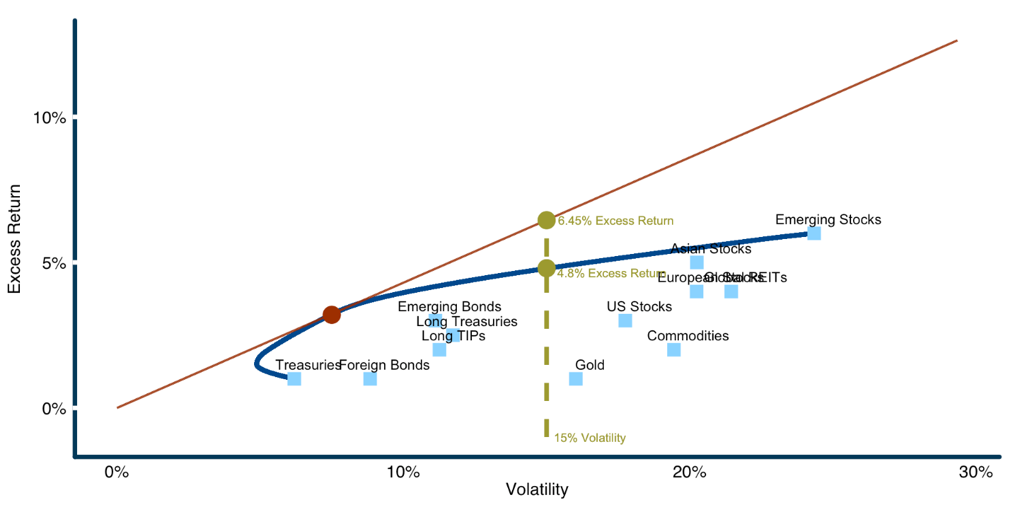
Source: ReSolve Asset Management. For illustrative purposes only.

Let’s examine a case where a “growth” investor wishes to maximize his rate of return given that he can tolerate 15% annual volatility, consistent with the historical risk character of a 70/30 global stock/high grade bond portfolio. Under typical conditions, this investor would be forced to push out the efficient frontier and take on a concentrated portfolio of equity markets. Figure 2 describes the composition of this portfolio.

Figure 2: Mean-Variance Optimal Portfolio at 15% Target Volatility Along Efficient Frontier

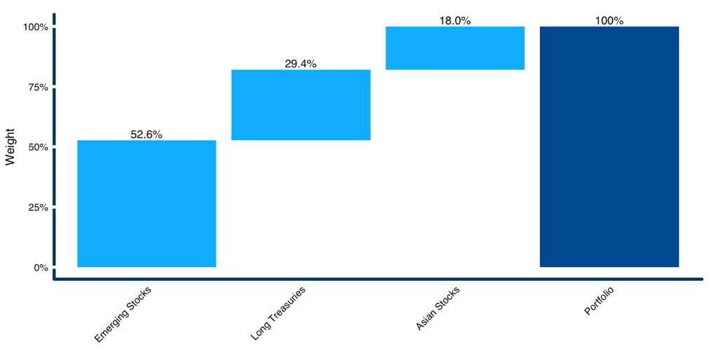
Source: ReSolve Asset Management. For illustrative purposes only.

Given the capital market assumptions above, to achieve the highest return possible at no more than 15% volatility would require that he hold 29.4% long Treasury bonds, 18% Asian stocks, 52.6% emerging stocks, since this is the most efficient portfolio at 15% volatility.

This portfolio would be expected to earn 4.8% annual excess return, highlighted with a gold point on the efficient frontier in Figure 1.

Leveraging the diversified portfolio

Now consider an investor who is liberated from the no-leverage tyranny imposed by the efficient frontier. He can choose to own the more diversified mean-variance optimal portfolio described in Figure 3, and borrow (with margin or futures or other derivatives) to purchase more units of the portfolio using leverage until he achieves his target volatility. Again given our working capital market assumptions, this portfolio would be dominated by emerging bonds, long Treasury bonds, and Asian stocks.

Figure 3: Maximum Sharpe Ratio Portfolio

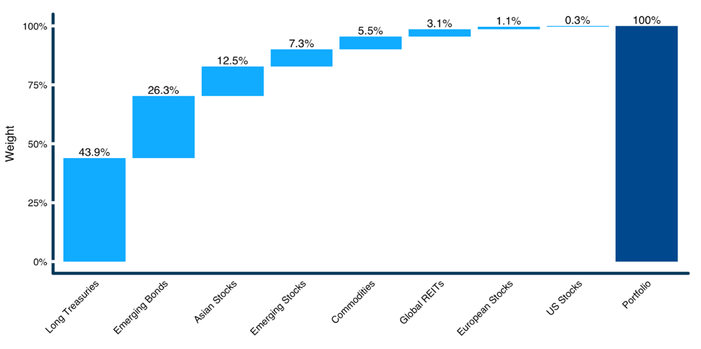
Source: ReSolve Asset Management. For illustrative purposes only.

Leverage is a foreign concept for many novice investors. But readers with an open mind will recognize that by using a prudent[7] amount of leverage to invest in the maximum Sharpe ratio portfolio, they can now take advantage of investments that earn their premium during very different market environments, and from diverse economic regions.

The concentrated equity investor would only expect to earn attractive returns during periods of sustained economic growth, benign inflation, and abundant liquidity. However, the maximum Sharpe ratio portfolio in Figure 3 contains Treasury bonds, which are designed to benefit during deflationary growth shocks; emerging bonds, which would benefit from an increase in credit quality among emerging countries, as well as potential currency tailwinds; and equity markets from around the world.

Aside from the benefits of broader diversification, the choice to leverage the maximum Sharpe ratio portfolio in Figure 3 provides an opportunity to earn 6.45% excess return, a full 1.65 percentage points more per year than the investor can expect to achieve by moving out the frontier. This point is also highlighted on the CML in Figure 1.

To close the loop, investors who focus their trend trading on equity indexes because the equity-risk premium is of a larger magnitude than other premia are missing the point. Under reasonable assumptions about the general relationship between risk and return, a diversified portfolio will produce considerably greater return per unit of risk. When scaled up the CML using prudent amounts of leverage, this leads to a higher absolute return, period, than a concentrated position in equities.

Of course, the benefits of diversification grow in proportion to the number of alternative sources of return that are available. Diversification is the key.

The key is diversification

Notwithstanding the benefits of diversifying into uncorrelated markets outside of equities, many investors start their investment journey with a myopic focus on equities. Upon discovering the benefits of trend following, they often spend years applying the techniques to time a major stock index, such as the S&P 500 or their local market.

In this section we will continue to focus on equity market-trend following. We’ll examine the performance of a representative trend-following strategy applied to 15 global stock index futures.

First we’ll observe the performance of the trend strategy when applied to the individual markets. Then we’ll demonstrate the monstrous advantage that is available from trading a diversified strategy of all equity indexes. Finally, we’ll expand our horizon to include assets outside of equities, and unleash the true potential of diversified multi-asset trend-following.

Trend following on individual stock index futures

We first examine the distribution of trend-following performance when applied to individual equity index futures, relative to the performance that can be achieved by trading a diversified basket of equity index futures. To keep things simple, we examine the performance of a simple moving-average trend-trading strategy, based on a 200-day (~10 month) lookback horizon. The strategy will hold a market long when its price is above its moving average, and exit when price falls below.

Let’s first observe the growth profile of our toy trend strategy when it is applied to futures tracking several major equity markets around the world.

Figure 4 plots the growth trajectories for each equity index futures market. S&P 500 futures started trading in 1983, and other markets were introduced over time. To account for the fact that some markets have less time to compound (because they come into existence later), we bring each market into existence at the current level of the S&P 500 strategy. Thus, the terminal value for each strategy in Figure 4 offers a meaningful indication of relative performance.

Figure 4: Growth of $1: Simple 200 Day Moving Average Long/Flat Trend Strategy Applied to Futures on Major Equity Indices

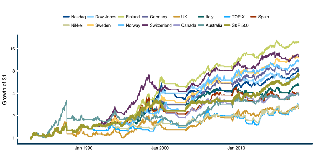
Source: Calcuations by ReSolve Asset Management. Data from CSI Data. Growth of $1 from executing long/flat 200-day moving-average trend strategies on equity index futures scaled to ex post 20% volatility.

There is a large dispersion in results across markets. Japanese investors trading the TOPIX or the Nikkei fared much worse than Finnish or Swiss investors trading exactly the same strategy. In fact, the worst strategy grew $1 to just over $2 in 35 years, while the best strategy turned $1 into over $16.

Perhaps surprisingly, while the trend strategy improved risk-adjusted performance relative to a buy and hold strategy for the majority of equity indexes, investors in Commonwealth countries (UK, Canada and Australia) experienced lower absolute and risk-adjusted returns by following trends.

In our toy example, if the investor chooses to run a trend-following strategy on just one equity index, he has equity assets to choose from. Assuming the investor chose one equity index to trade at random, the best estimate of the investor’s performance is the median performance among all strategies.

Importantly, it is the median that matters to one investor who chooses just one strategy, not the mean, because the investor can live just one life, and has chosen not to take advantage of the law of large numbers[8].

A diversified global equity index trend-following strategy

What many investors miss is that, absent extremely confident views about which market will outperform in the future, investors are better off trading all of the markets at once.

Let’s consider a more humble investor that is focused on investing in equities, but cannot decide which market(s) to trade. Instead, he chooses to trade all of the equity index assets as part of one diversified strategy.

The “portfolio” quantity in Figure 5 reflects the performance of this diversified strategy relative to the median strategy. Critically, the diversified strategy benefits from the fact that the returns from each of the individual strategies are not perfectly correlated. In other words, they diversify one another.

Figure 5 compares the Sharpe ratio of a diversified trend strategy, which trades all equity markets, against the median performance of trend strategies over the 15 equity index futures.

An investor choosing a market to trade at random would have expected to experience a Sharpe ratio of 0.45, while an investor who traded all markets as a diversified trend strategy would have achieved a Sharpe ratio of 0.76. The difference between the “median” and the “portfolio” performance is the bonus that an investor accrued from taking advantage of this diversification.

Astonishingly, investors who chose to diversify would have produced 1.69x the return per unit of risk relative to an investor trading one random market. This diversification bonus is so large that the “portfolio” strategy surpasses the risk adjusted performance of all but one of the individual strategies[9]. Which means an investor would have had to be better than 93% accurate in choosing which index to trade in advance in order to achieve better performance than one could generate from simply diversifying across all of them.

For those focused on U.S. stocks, it’s worth noting that the diversified strategy dominated trend trading on the S&P 500, with a Sharpe ratio of 0.51, by almost 50%.[10]

Figure 5: Marginal Sharpe Contribution from Diversified Long/Flat Trend Trading Across Equity Markets vs. Median Performance by Individual Market

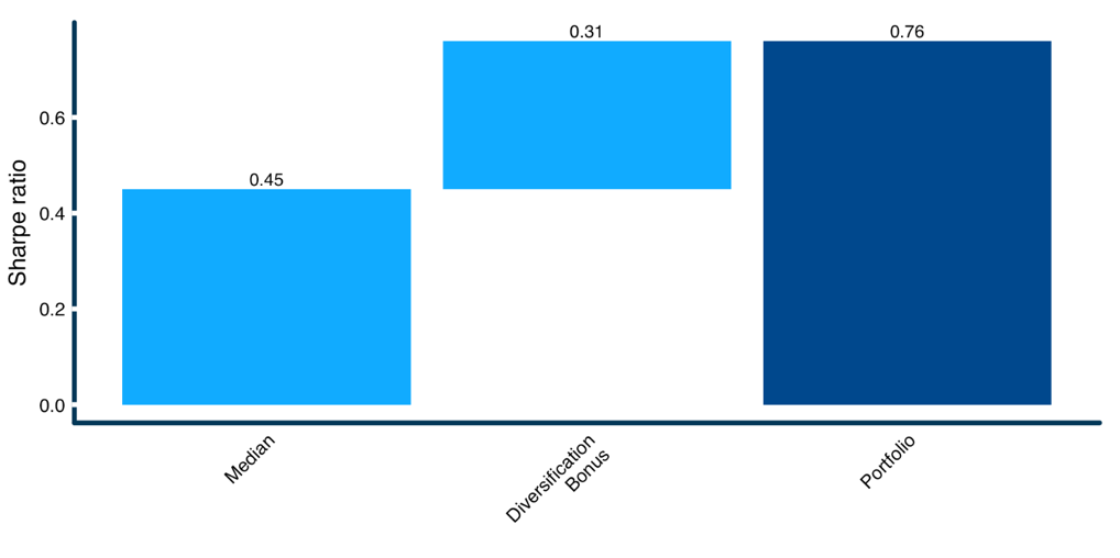
Source: Calcuations by ReSolve Asset Management. Data from CSI Data. “Median” is the median Sharpe ratio of long/flat 200-day moving-average trend strategies applied to individual equity index futures. “Portfolio” is the Sharpe ratio of a strategy that trades all of the equity index futures markets as one aggregate strategy. Diversification Bonus is the improvement in performance from trading all equity index futures as a diversified strategy instead of choosing one market to trade. Performance does not account for fees, transacation costs, or other factors which may impact performance. For illustrative purposes only.

Diversification in bonds, currencies and commodities

We mentioned above that the concept of diversification extends (obviously) to other asset classes besides equities. The fact is, it rarely pays to focus your efforts on any one market, in any asset class.

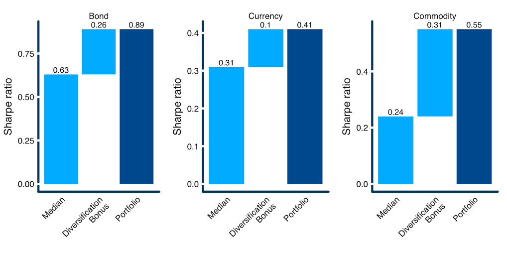
Let’s expand our domain of analysis to include six bond futures, seven currency futures, and twenty commodity futures. Figure 6 describes the diversification bonus from choosing to trade all markets in each category, rather than trading any single one.

The commodity asset category provides a particularly interesting case study. Long/flat trading based on a simple 200-day moving average has not been a particularly profitable strategy for individual commodity markets over the past few decades. The median Sharpe ratio for trend strategies across twenty commodities is just 0.24.

However, commodity markets are generally uncorrelated with one another. That means that there is a large advantage to running even relatively ineffective strategies “across the board.” Incredibly, an investor would have achieved 2.29x the return per unit of risk relative to an investor trading any one random commodity market.

Figure 6: Marginal Sharpe Contribution from Diversified Long/Flat Trend Trading Across Major Asset Categories vs. Median Performance by Individual Market Within Each Asset Category

The power of diversified trend following

Now that we’ve quantified the diversification bonus for investors who are concentrated in any one asset category, we conclude by expanding the trend strategy to trade all assets from all categories at once. This is obviously where the rubber hits the road, since professional trend followers use all the instruments at their disposal to achieve the largest diversification bonus possible.

Figure 7 describes the gargantuan bonus available to investors who understand the power of combining trend-following with diversification across all major asset categories. It’s shocking to see that diversification alone can transform many independent strategies with low Sharpe ratios on their own into a diversified strategy with long-term performance that rivals even the most successful markets and hedge funds.

Figure 7: Marginal Sharpe Contribution from Diversified Long/Flat Trend Trading Across All Markets vs. Median Performance by Individual Market

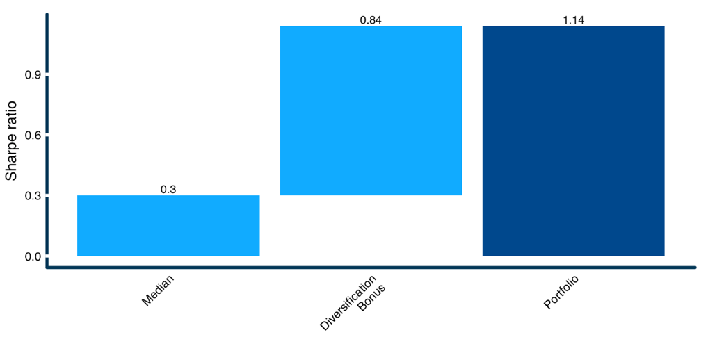
Source: Calculations by ReSolve Asset Management. Data from CSI Data. “Median” is the median Sharpe ratio of long/flat 200-day moving-average trend strategies run on each individual market across all asset categories. Markets are weighted using ex post inverse volatility. “Portfolio” is the Sharpe ratio of a strategy that trades all markets in all categories as one aggregate strategy. “Diversification Bonus”” is the improvement in performance from trading all markets as one aggregate strategy instead of choosing one asset to trade. Performance does not account for fees, transacation costs, or other factors which may impact performance. For illustrative purposes only.

Summary

For natural reasons, many novice investors and advisors try to harness the power of trend following to trade their favorite equity index. But this misses the point. By trend trading a single index, investors are extremely vulnerable to the probability of choosing an equity market with low forward returns, unproductive trends, or both.

The true benefit of trend following is only realized when investors take advantage of the extreme liquidity and diversity of global futures markets to trade a wide range of markets across all major asset categories. Our analysis shows that an investor would have achieved more than double the risk-adjusted performance of a median equity trend strategy by trading a diversified strategy across many diverse markets.

Traditionally, many diversified futures funds were only available to qualified investors. This barrier has lifted over the past few years with the introduction of liquid alternatives, as several private funds have been “converted” to traditional mutual funds. Catalyst and Rational Funds have been especially active in making top futures strategies available to everyone. Even better, gains on futures receive favorable tax treatment, and futures funds are often extremely capital efficient.

[1] Siegel, Jeremy J. “Stocks for the Long Run, 2nd ed.”, McGraw-Hill (1998)

[2] Covel, Michael W. “Trend Following: Learn to Make Millions in Up or Down Markets”, FT Press (2009)

[3] Schwager, Jack D. “Market Wizards”, HarperCollings (1989)

[4] Small investors may have skill and certain advantages (i.e. liquidity, mandate flexibility, portfolio agility, long-term thinking, etc.), but they also pay egregious fees for margin, typically cannot effectively access futures and swaps markets, and either a) pay onerous commissions or b) trade for “free” but get killed on execution because the broker sells their flow for rebates. Remember, the broker has to get paid somehow…

[5] Paper can be found here

[6] NOT official ReSolve estimates.

[7] Some readers might wonder about the term “prudent” referring to leverage. For context, the average leverage ratio for the S&P 500 is 1.7x since 1995, which means there is $1.7 of debt forever $1 of equity.

[8] To gain a deeper understanding of the concept of ergodicity and the difference between ensemble mean and finite time mean, please see this article.

[9] I know, I know, you all would have known to trade Finnish index futures in advance, so this point is moot.

[10] Many investors have probably examined the performance of a 200 day moving average strategy on the S&P 500 using index data. It may surprise aspiring quants to learn that the exact same strategy run on the S&P 500 total return cash index produces a substantially higher Sharpe ratio over the same period. Please do not learn the wrong lesson! Given very small changes in the exact path of returns, we could just have easily have seen that the futures strategy outperformed the cash index strategy. This dispersion in performance highlights the extreme fragility of this type of strategy run on just one index, and the sensitivity to path dependence.

Read more articles by Adam Butler