A paper by Campbell R. Harvey, Yan Liu, and Heqing Zhu with the unexciting title “…and the Cross-Section of Expected Returns” has been drawing a lot of attention recently. This is not only because of the paper’s startling revelation that at least 315 “factors” of investment returns have been discovered through multiple regressions and published in hundreds of articles and working papers. That phenomenon was already characterized in a 2011 paper by John H. Cochrane and called a “zoo” of factors. It is also because Harvey et al.’s work sounds the same alarm for finance research that was sounded in 2005 for medical research in a famous article by John P. A. Ioannidis, “Why Most Published Research Findings Are False.”
Harvey et al. claim that “most claimed research findings in financial economics are likely false.” I’ll explain how they arrived at that conclusion by looking at the ongoing search for factors that influence investment returns. Let’s begin by understanding the statistical tests that are used to determine whether or not a purported factor is the result of random “luck.”
What are factors?
A factor is any item of data that can be put into correspondence with the rates of return on a security or a portfolio of securities.
Let’s call that item of data x, and let’s call the monthly return on the security or securities r. Imagine two columns of numbers: the values of x and the values of r. Each value of x, the factor, corresponds to a value of r, a monthly rate of return. The value of x and the value of r might both be for the same month or for the same security. Or x and r might be for different months.
A factor could be a macroeconomic variable, like monthly inflation, interest rates or unemployment. In that case, a monthly return on the portfolio or security could be put into a correspondence with, say, the value of the macroeconomic variable in the preceding month. Imagine a column of monthly returns on a portfolio next to a column of unemployment rates in the previous month.
Alternatively, a factor could be a feature of the corporate security itself or portfolio of securities. For example, a factor could be the size of the corporation, the corporation’s price/earnings ratio or book value/market value ratio. Imagine a column of rates of return on all stocks in a given month next to a column of the price/earnings ratio of the company issuing the stock.
Whatever the factor is, the idea is to see if it bears a numerical relation to the corresponding rates of return when the two variables are lined up that way. A correlation coefficient would be one way to see if the data exhibits a numerical relationship. An equivalent method – one that has become standard – is to run a regression of the rates of return on the “factor” variable.
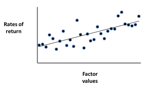
A regression is what is known to high school students – at least it was in my high school – as a least-squares fit. It results in a line with a slope and a y-intercept (Figure 1).
Figure 1.

The slope, often labeled with a “beta,” is supposed to represent the relationship. If the beta is zero, there is no apparent relationship (at least not a linear one). If beta is large – either a large positive or a large negative slope – there is a relationship.
The standard admonition must be repeated, however: it is not known what the nature of that relationship is. For example, a numerical relationship such as that depicted in Figure 1 does not establish a causal relationship. It is, nevertheless, common practice in finance research to ignore this admonition by saying that the factor “explains” the rates of return.
Figure 1 shows only a simple linear regression – one set of rates of return against one factor. It is also possible to run a multiple regression – one set of rates of return against more than one factor. Imagine three or more columns of numbers lined up next to each other. It is harder to visualize than the simple graph in Figure 1 because the least-squares fit becomes a plane instead of a line.
If you line up those columns in Microsoft Excel and highlight them, then select from the Data menu the Analysis option (if you have activated it) and select “Regression” – Presto! You’ll have run the regression in about two seconds.
The point is that if you had the numbers for many factors lined up in your spreadsheets, you could run hundreds of regressions in a single day. And that’s if you just used Excel. If you wrote a program to do it, you could run many more. More people in finance than you may realize do that.
Hypothesis testing
The idea of lining up the factors with the one-month rates of return is to formulate a hypothesis that the rates of return depend in some way on the factors – and maybe can even be predicted by the factors, the Holy Grail of the investment world.
As many or most readers will know from statistics classes – but may have forgotten – there is a well-defined procedure for testing such hypotheses.
The procedure is as follows. You start by assuming that the rates of return don’t depend on the factors; that is, that the betas are zero. This is known as the null hypothesis.
But since – as can be seen from Figure 1 – the data are spread out in a random pattern because of unknown factors, they might accidentally fall in a recognizable pattern. They might accidentally make it look like a coefficient of the regression – a beta, a slope of the regression line – isn’t zero, even if it really is.
There are ways to estimate the probability that this could happen. The steeper the slope of the fitted line, the less likely it could have happened; the less spread out in a random cloud around the fitted line the points are, again the less likely it could happen.
The probability it could have happened at random – even if there is no relationship, that is, if the null hypothesis is true – is known as the p-value.
Conventionally, if this p-value is less than 0.05 (5 percent), it is common to say that the test rejected the null hypothesis at the 0.05 significance level. That allows the researcher to say that the null hypothesis was rejected in favor of the alternative hypothesis – that the rates of return did indeed depend on the factor – and that this result was significant.
Multiple testing
Now, remember that the p-value measures the probability that the slope of the regression line – the beta – could have come out looking steep because of randomness. If the p-value were 0.05, or one-twentieth, that means that if you conducted 20 tests, in all of which the beta was really zero, then on average, in one of the tests, you would get a p-value of 0.05 or less. In that case you would have proclaimed the null hypothesis rejected at the 0.05 significance level.
So what happens if researchers are conducting hundreds or thousands of tests? For each hundred tests in which there is in reality no relationship between the factors and the rates of return, they will declare that in five tests they found a significant relationship.
Harvey et al.’s paper addresses this problem. They go through the procedures that have been developed in the field of statistics to deal with what is called the multiple comparisons or multiple testing problem.
In each procedure, the way to deal with the problem is simply to raise the bar, making it more difficult to declare a null hypothesis rejected. The solution is not to allow a researcher to declare a result significant if the p-value was only 0.05 or less. The p-value might have to be 0.005 or 0.0005 or even 0.0000005 before it can be declared significant. It depends on how many tests are being done by researchers everywhere.
The problem is that we don’t know how many tests are being done because researchers rarely if ever disclose this in their papers. Harvey et al. own that they can only review what has been published in the literature, and there are undoubtedly many tests that have been carried out that have not been published. In fact, published literature is biased in favor of publishing research in which the p-value is low. Tests in which the p-value does not meet the test of significance don’t see the light of day.
And as we have seen, such tests could number in the thousands, even in the tens of thousands. For example, in an interview with Stanford economist Russ Roberts, Harvey pointed to an experience he had “at a high-level meeting, at one of the top 3 investment banks in the world.” A person at the company was presenting his research, “and basically he had found a variable that looked highly significant in beating the market, with a regression analysis… And it turned out that this variable was the 17th monthly lag in U.S. Industrial Production.” And Harvey said, “the 17th--where's that coming from?” And then the researcher basically said, “Well, that's the only one that worked.”
A large number of factor regressions like this are surely being done – an enormous number -- and we don’t know how many. Some of them are sure to “work.” But most of those that work are accidents of randomness. How shall we know which ones? Harvey et al.’s approach – the multiple-testing approach – of simply raising the bar of significance won’t suffice because there might be thousands upon thousands of tests being done, and most of the results have been placed off the record. Harvey et al. mention that in the field of medicine attempts to replicate previously published research are frequently performed and often fail to confirm the previous results. But in the field of finance, attempts at replication are uncommon. Research in the field is a free-for-all without adequate rules or discipline.
Is it impossible to raise the bar high enough?
Harvey et al.’s paper does not ask a crucial question: Is it even possible to raise the bar high enough? Is there perhaps a Heisenberg uncertainty principle in statistical research in finance, in which, when the signal-to-noise ratio – that is, the ratio of structure to randomness in the data – is too low, it will be impossible to distinguish spurious results from real ones?
The answer is yes, there is. Imagine a sequence of monthly rates of return. Now imagine a virtually endless array of series of factors that could be matched to that sequence – that is, that could be placed in a column next to it. Such a nearly endless array is easy to conjure by combining factors to create new factors for example, or by lagging them by one month, two months, …, 17 months, …, and so on.
Suppose now that there is a real relationship – a regression beta – of the sequence of rates of return against one of the factors. But in each case there is a high level of noise.
Here is what will happen. Because of the noise – and no matter how high the significance bar is raised – a regression of the rates of return against some one of the factors will produce a significant result. But the chances, if the signal-to-noise ratio is low enough, that the factor so identified will be the one that actually does bear a relationship to the sequence of rates of return will be arbitrarily low.
The identification of spurious factors will be inevitable even if one (or perhaps more) of them really does affect rates of return.
But that’s only the beginning of the problems when it comes to investments
All of this rests on the assumption that relationships between factors and rates of return – if they exist – are persistent. That is, that they persist from one time period to another. This assumption is warranted in almost all scientific fields. If a result of a combination of physical forces is convincingly discovered in experiments, it will work in the future too. If a vaccine is developed that prevents a disease for test subjects, it will work even if everybody uses it.
These assumptions are completely unwarranted in the investment field. If an investment strategy that beats the market is discovered and verified – even if it is not a spurious discovery – it will not work for everybody. It cannot; it is tautologically obvious that not everybody can beat the market. Hence, a strategy that is identified as effective, correctly or not, must, at some point, if it becomes popular and widely adopted, stop working and may even reverse to become a bad strategy.
What, then, are all those people running all those regressions doing?
They are creating an impression; an impression of diligent, technologically sophisticated research.
This is called busywork. And the most highly compensated busywork in the world it is.
Michael Edesess, a mathematician and economist, is a visiting fellow with the Centre for Systems Informatics Engineering at City University of Hong Kong, a principal and chief strategist of Compendium Finance and a research associate at EDHEC-Risk Institute. In 2007, he authored a book about the investment services industry titled The Big Investment Lie, published by Berrett-Koehler. His new book, The Three Simple Rules of Investing, co-authored with Kwok L. Tsui, Carol Fabbri and George Peacock, has just been published by Berrett-Koehler.
Kwok L. Tsui is a distinguished statistician and Head of the Systems Engineering and Engineering Management department and Chair Professor of Industrial Engineering at City University of Hong Kong.
Read more articles by Michael Edesess and Kwok L. Tsui