Do house prices experience periodic bull and bear markets like the stock market? Or are they stable in real (inflation-adjusted) terms most of the time, with big disruptions once or twice in a century? Two popular house price series tell these very different stories. Knowing which is better will lead to superior investment outcomes and improved policy decisions.
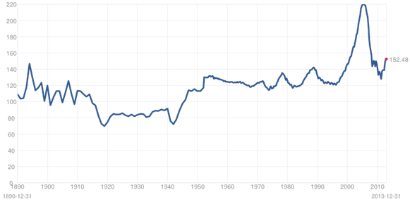
Karl (Chip) Case, of Wellesley College, and the Nobel Prize-winning Yale professor Robert Shiller, have constructed the most widely-known suite of indices, which are now part of the S&P index family. Here is the Case-Shiller national house price index in real terms from 1890 through December 2013:
Figure 1
Case-Shiller National House Price Index in Constant Dollars, 1890-2013

Source: http://www.multpl.com/case-shiller-home-price-index-inflation-adjusted/
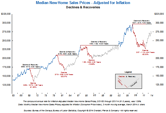
And here is a house price series distributed by the data firm of Crandall, Pierce & Co., consisting of the median new home sales price in constant dollars collected by the U.S. Department of Housing and Urban Development. (For brevity, we call this the “Crandall” series.)
Figure 2
Crandall, Pierce Median New Home Sale Prices in Constant Dollars, March 1963-March 2014.03
Source: Crandall, Pierce & Co., Libertyville, IL. Reprinted with permission.
Could any two charts describing the same underlying phenomenon look more different? In the Case-Shiller chart, there was one great bear market in the last 50 years, from late 2006 to early 2012, following a massive price expansion or bubble.1
In the Crandall chart, however, bull and bear markets have alternated in a remarkably regular pattern. All of the bear markets represent losses of roughly 20%, with the crash of 2008-2011 only a little worse than the three other housing bear markets that occurred in 1968-1970, 1979-1982, and 1988-1992. The Crandall chart also shows real prices rising pretty smartly – 1.35% per year – while the Case-Shiller chart shows a much slower rise.
Note that the two price series do not purport to measure the same thing. The Crandall data are for new houses only; the Case-Shiller data are intended to reflect the entire stock of housing capital.2 The Crandall data are for a median house, the size and quality of which are constantly changing; Case and Shiller explicitly adjust for changes in the size and quality of a house. There are many other differences, so it’s understandable that the two series disagree somewhat – but they’re both intended to track house prices, so the contrast between them is striking and troubling.
Which chart provides a more reliable picture of housing-market returns as experienced by the typical investor?
We should care because the return and volatility of individually owned real estate has profound investment and public policy implications.
Investment implications of house price return and volatility
Paul Samuelson said we are born short a roof over our heads. Thus, if we buy a house – one house – it's a hedge, not a speculation. The value of the liability (the need to have a house) moves with the value of the asset (the house). For this investment we do not care much about the return and volatility characteristics; we are just prepaying a liability.
But if we speculate in real estate by buying houses or other properties to rent out, they become a portfolio asset like any other. We need to know the expected returns, volatility and correlations with other assets. The Crandall data make housing look like a normal capital asset, one that fluctuates with expected cash flows and discount rates, and that has a standard deviation typical of assets having similar expected returns.
The Case-Shiller data, however, make housing look like a magical asset until it crashes; it has a decent return with almost no volatility. The return is decent because of the receipt of rent. Both the Case-Shiller and Crandall series are price-only, leaving out income from rent net of expenses, which is the primary source of profit for real estate investors. Independent studies have shown that total returns on unleveraged real estate are between those of stocks and bonds.3
The Case-Shiller and Crandall charts, then, present two very different investment profiles and would cause you to behave very differently as a real estate investor depending on which chart is accurate.
Public policy toward real estate
If the Crandall data are correct, the housing crash of 2006-2012 was a normal bear market, a little more severe than the others but not qualitatively different. If so, then the policies preceding the crash were not so bad. Subprime mortgages, loose appraisal practices, and so forth are part of the ordinary workings of a competitive market where people try different things to sell houses and lend money.
But if the Case-Shiller data are correct, we would want to avoid repeating the policies that led up to the crash at all costs. Homeowners who bought (or took out new mortgages) at the top may never recover. If the bubble and subsequent crash in the Case-Shiller data are due to policy errors, these errors are unconscionable.
Starting points
We came into this investigation with some biases, and it’s healthy to disclose what they are. On one hand, we believed at some level that there is nothing new under the sun. Every capital market phenomenon has an antecedent, or many of them. Real estate values, hence prices, have been fluctuating since expected cash flows and discount rates have been fluctuating – that is, forever. There is no fundamental reason why real estate should not look like any other asset, and in the Crandall chart – which is a pretty picture – it looks very much like one, with bull and bear markets and short-term volatility.
But we were also pretty sure that real estate in the 2000s experienced a crash that was qualitatively more severe than a normal bear market. The pain was far worse and extended far more widely than in previous episodes. Was this just a matter of too much lending to buyers who were poorly positioned to take such risk? Probably not. The percentage decline in real estate prices, we believed, was at least partly to blame for the feeling that there had been a real estate depression.
Comparing the two series
Let’s compare the two series across a number of dimensions.
Long-run rate of return
Before delving into the differences between the Crandall and Case-Shiller series, let’s note the similarities. The long-term rates of return do not seem radically different: 1.5% per year for Crandall and 0.5% for Case-Shiller (both are real, and price-only). But this 1% per year “spread” is economically significant when compounded over long periods of time.
Houses have grown substantially in size and quality over the period studied, so part of the 1.5% annual increase in the Crandall series – which is just a median real new-house sale price – is obviously due to that increase. The Case-Shiller series explicitly adjusts for quality changes and still shows a 0.5% real capital gain, so we accept that lower rate as correct.
Timing of bear markets
The timing of three of the bear markets (1979-1982, 1988-1992, and 2006-2012) is also similar.4 But, oddly, the Crandall series shows a sharp bear market in the late 1960s that is completely missing from the Case-Shiller data. Overall, the short-term volatility of the Crandall series is higher. But the biggest and most important difference is that the crash of 2006-2012 is much worse in the Case-Shiller data, representing a 43% decline from the peak, compared with a 23% decline from the peak in the Crandall data. The crash according to Case-Shiller took the real price index all the way back down to its level in June 1998, at which time the index had been essentially flat (with some volatility) for more than 30 years. In his interpretive writing, Shiller has emphasized the flatness of the real price appreciation curve, arguing that investing in houses has been a poor way to make money in the long run.5 We’ll return to this theme later.
The great bubble bursts
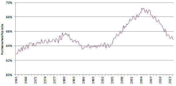
In 2006-2012, however, there was a perfect storm of bad luck, bad policy and stupidity. Homeownership, measured by owner-occupants as a fraction of total households, had advanced to historical highs, with the marginal buyer being very marginal indeed. (Homeownership peaked at 69% of all households, about five percentage points above the long-run average.) House prices were sky-high, nearly double their real long-term average. Incomes plummeted as the Great Recession spread from the financial sector to the rest of the economy.
Teaser rates and low interest-coverage requirements had enabled borrowers to qualify for mortgages, but not to service them when the teaser rate expired and the normal interest rate began to be applied. (One might think lenders would take this into account, but loan originators were being paid on the volume of loans made, not on the dollars paid back.) As the American Enterprise Institute economist Peter J. Wallison has pointed out, Fannie Mae and Freddie Mac became subject to increasingly onerous mandates to make a large percentage of their loans to low-income and “very low income” households.6
The upshot was a Case-Shiller index that fell almost by half, back to its early 1998 level in real terms (also its 1977 and 1986 levels and a few percentage points above its 1965 level). This crash, which thus wiped out almost a decade of exceptional profits for homeowners, really was qualitatively different (and much more severe) than the others.
How the Crandall and Case-Shiller series are constructed
While the Crandall data (real median new-home sale prices) are pretty transparent, as are their limitations, the Case-Shiller data are more complex. For 1953-1975, Case and Shiller use the Home Purchase Component of the U.S. CPI, collected by the Bureau of Labor Statistics and covering prices for homes where the age and square footage was held constant. This component was eventually discontinued for the CPI due to several well-known deficiencies acknowledged by Shiller.7 Given those deficiencies and the anecdotal evidence of the time,8 one can make a pretty good case that the short, sharp housing bear market of 1968-1970 really happened, followed by a quick recovery. There is also little question that the bear markets of 1979-1982 and 1988-1992 really happened, although the latter was concentrated in specific regions of the country.
From 1975 to 1987, Case and Shiller use the House Price Index from the Federal Housing Finance Agency (FHFA), formerly the Office of Federal Housing Enterprise Oversight (OFHEO). This is also a repeat sales index, which controls for quality changes. Starting in 1987, Case and Shiller constructed their own data, and their method from 1987 to the present was used in the Case-Shiller series going forward.
We care about both history and the future, for slightly different reasons. Recall our original reason for asking the question, “Which index is better?” We want to know whether housing is a conventional volatile capital asset. To answer this, we need to know history – we need to know whether housing experienced one bear market or four in the last half-century. It is clear that three of the four shown by Crandall did happen, and the evidence for the first one is mixed. Real estate is indeed a capital asset that fluctuates with changes in expected future cash flows and discount rates; how could it be otherwise? There are no magical assets, no assets that present reward but little or no risk.
But the most recent crisis has many features distinguishing it from all others (except the Great Depression), and we need to know how bad the crisis was, because it could happen again and it’s important to know how bad things can get. Therefore, we are curious whether the 2006-2012 crash involved a 23% or a 43% housing price decline.
This question isn’t decided by the relative accuracy of the Crandall and Case-Shiller series pre-1987, because Case and Shiller’s data sources before that date are no longer used. We simply want to know which one is the more accurate measure of price return today: The median new-home sales price used in Crandall or the repeat-sale regression constructed by Case and Shiller.
And the answer to that question is almost certainly Case and Shiller. During a housing depression, there aren’t many new homes, and those that are sold may have special characteristics – they may be cheap or expensive, or located in a part of the country that is little affected by the depression. Existing homes are a much deeper market, and when prices “gap down” for a seller, the market price is also likely to have gapped down for houses that are not for sale, or that are hard to sell and that thus do not record repeat-sale prices.
The countervailing bias in Case-Shiller is that their index is transaction-weighted and boomtowns such as New York, San Francisco, Chicago and Washington have an outsized influence on the index. Housing prices in these locations almost certainly rose more and then fell more than the national average. Therefore the 43% decline may be somewhat overstated. But it is probably closer to reality – to a typical homeowner’s experience – than 23% is.
The 2006-2012 downturn was qualitatively worse than the others
Thus, this most recent housing downturn was quantitatively different from the earlier ones. Notably, it was also qualitatively different:
Pre-World War II events aside, the nationwide character of the 2006-2012 crisis is unprecedented.9 While there were regional differences, big price gains accrued along the whole West Coast, in Arizona, Nevada, Florida and practically the entire Northeast. These areas taken together represent a majority of the U.S. population. Declines in smaller regions, such as those occurring in previous housing bear markets, are much less serious.
-
Nominal versus real effects: Because of low inflation and low down payments in 2006-2012, many more homeowners were underwater than in previous downturns. The behavioral effects of being underwater are huge, especially for unseasoned homebuyers who were recently renters. They walk away from their mortgages in much greater numbers than long-term property owners who can afford to keep paying the mortgage while they wait for the recovery. Moreover, when inflation is low, the financial burden of a fixed monthly payment doesn’t go down in real terms very quickly, compounding the problem.
Ownership base: As suggested above, extending the ownership base causes the pain of any given downturn to become dramatically amplified. Not only were new owners in more vulnerable groups than before, many seasoned owners borrowed additional funds in the run-up and came to have financial characteristics resembling the newest owners. Figure 3 shows how the base of owners had grown leading up to the crisis. While those last few percentage points in the ownership base may not seem all that significant, remember that most of the people who wanted and could afford houses already had them, so those added last to the ownership base were marginal indeed.
Figure 3
Homeownership rate in the United States, 1965-2014
Source: U.S. Census Bureau
With all this information in hand, let’s compare the 2006-2012 bear market to the one in 1979-1982, which was similar if one uses the Crandall data. (We do not know enough about 1968-1970.) The big difference is that in 1979-1982, inflation was high (good for borrowers), nominal prices were not falling (just real prices), ownership rates peaked at “just” 66% (vs. 69% in 2007), and homeowner leverage was much lower. Therefore, even if we take the “Crandall” 23% decline in 2006-2012 at face value, instead of the gargantuan 43% of Case-Shiller, the recent crisis should have been much worse than the one in 1979, simply owing to its idiosyncrasies.
In other words, even if we agree that the recent crisis was worse than the others, it doesn’t immediately follow that Case-Shiller is the better index for representing reality simply because it recorded a larger drop. Even if the real percentage price drop was the same as in 1979-1982, we should have anticipated greater pain!
Is a house a hedge or a speculation?
As the Shiller real capital gain data show, it’s hard to make much money by buying and holding a house. Huge profits in boom cities (many of which were surprisingly cheap a generation or two ago) are offset by losses or stable prices in declining cities, towns, and rural areas. Moreover, nominal profits often translate to real losses; many homeowners would have done better in the S&P 500 or the bond market.
One hears stories about the huge fortunes made – but not the losses incurred – in residential real estate, for the same reason one hears stories about fortunes made in the stock market: people brag about their gains but keep quiet about their losses. On average – although few homeowners got the average return; more typically getting much more or much less – residential real estate provided a real capital gain of one-half of one percent a year over 1890-2014 (or 1953-2014). That’s not much of a return.
What these owner-occupant-investors did get, however, is a place to live. If we think of housing as a consumption good with two principal ways of contracting for it (renting and owning), we can begin to make sense of housing decisions. Most people buy or rent the best housing they can afford, not because they think it’s the best investment (it’s too undiversified), but because they want to live in it. This is the right way to think about deciding what housing to buy or rent and how much to invest in it.
In finance lingo, the receipt of a place to live is the income return, or imputed rent net of expenses, on an owner-occupied real estate purchase.10 As in the bond market and to some extent in the stock market, the income return is historically the greater part of the total return.11 When imputed rent is added to the capital gain return on a house, the total return is competitive with that of a stock-bond portfolio, as noted earlier. Prospective homeowners should choose their housing first and foremost on the basis of its consumption value, and only secondarily on the basis of how good an investment it seems to be.12 But the household’s main investment decisions should be elsewhere – in stocks, bonds, cash, and most importantly human capital (earning power).
Bringing this discussion back to Samuelson’s comment at the beginning about housing being a hedge, we’re saying that the hedging value of housing is much more important than the speculative value. And the income return is much more important than the capital gain return. We are not only born short a roof over our heads – many of us are born with the talent to make the roof we hold as an offsetting long position quite nice. And we’re all born lucky in that we live in an advanced technological society where the rewards to such talent can be substantial. Homeowners would do well to remember their good fortune in this regard.
So which is the better index?
It depends. (Surprise.)
For estimating the long-run rate of return, the Case-Shiller data are better constructed (but imputed rent, net of expenses, must be added to estimate the total return). The long-run rate of return estimate helps us with the decision of whether to invest in housing as a speculation or just a hedge, and how much to hold in housing versus other investments.
Moreover, for figuring out the magnitude of moves in the overall housing market, the Case-Shiller data are better. They better represent a basket of well-diversified properties across quality points and geography. The Crandall series is pretty naïve (just new homes, without quality adjustments – and just a median price).
But for estimating volatility and determining how often and how severe housing bear markets have been, the Crandall data have an edge. The Case-Shiller data before 1987 look smoothed, and probably are. In contrast, the evolution of prices in the actual real estate market is not smooth. People do experience, and sometimes realize, losses. In fact, the reluctance to realize losses by selling (or actual inability to do so because of the cash that would be needed at closing) dampens volatility as measured by sales prices, while the larger “true” volatility is given by the price an owner would have received at any given time if he or she wanted to sell.
Finally, we believe that the Case-Shiller data more accurately reveal the depth of the 2006-2012 housing depression.
Policy implications
If we believe in the greater severity of the 2006-2012 bust, then the Case-Shiller indices captured the pain better. This conclusion puts the policy decisions leading to that situation in a very poor light. There is plenty of blame to apportion. We don’t want to go too far back – government-created biases towards homeownership are decades old and didn’t create a housing bubble, at least not right away – so let’s look at more contemporary concerns.
A perfect storm of stupidity
It’s been said that love makes you stupid; and the love of money, especially of potential future gains, can make you even stupider. As we said earlier, we experienced a perfect storm of stupidity:
-
Government failed. Strongly influenced by Congressional mandates, Fannie Mae and Freddie Mac executives and shareholders made huge profits from fishy lending. It was like parents finding a wild party going on at home and, instead of sending everyone else home and grounding their children, they open up the liquor cabinet and start serving shots.
Regulators and the Fed failed. By taking financial institutions at their word, instead of relying on their own analysis, regulators allowed banks and non-bank financial institutions to build astonishingly bad balance sheets. We understand that regulators are understaffed and outgunned by market participants, but the well-heeled Fed is the regulator of the banking system and they didn’t seem to have a clue that the system they were overseeing was unsound.
-
Rating companies failed. They sell ratings to issuers, who can comparison shop for the best rating. Given that structure, we’re not sure why anyone uses the ratings. The agencies are full of conflicts of interest and seem only able to forecast the past.
-
Financial companies failed. There was some fraud – but, for the most part, the massive losses of the banks and mortgage lenders were due to the myopic behavior of their leaders, who were focused on short-term gains and blind to risks that were obvious (and hedgeable) in retrospect. Ill-conceived incentives and bonus structures explain the poor quality of on-the-ground credit delivery, but that criticism is not appropriate for the CEOs, who should have known better than to bet their firms on the hyperinflated mortgage market.
Households failed: While a few households can make a creditable claim that they were misled, when you borrow money you have to have a plan for paying it back. Too often, borrowers now portraying themselves as victims were ecstatic at receiving an unexpected loan “bounty.” Nevertheless, it is worth noting that households took the lion’s share of the losses.
Investors failed: For the bubble to inflate in the first place, somebody had to buy the mortgage-backed securities that would turn out to be nearly worthless, providing the ultimate financing for the houses. The “somebody” turned out to be money market funds, corporate bond funds, pension and endowment funds, hedge funds – those long-term stewards of capital who are supposed to balance risk against the hope of return and build sensibly diversified portfolios. Ha!
What should have been done differently?
We dislike government intervention. We believe markets can efficiently assign resources if they can work freely. In practice the conditions for a free and efficient market are seldom fully met, but even so, market solutions are usually better than other solutions. One cannot, however, ignore externalities or a distortion of the cost/benefit relationship caused by an imperfect allocation of property rights.
Take Fannie Mae and Freddie Mac. If the U.S. government took seriously the responsibility that came with its implicit guarantee of these agencies, it would not have allowed them to lower their lending standards, which were accommodating by design in the first place.
Would that have stopped the bubble? In the 1950s and early 1960s, we had low interest rates, low down payments (with FHA and VA mortgages), and marginal buyers (young World War II veterans) but no bubble. The real cost of housing actually trended down. In the 1980s, we had mortgage securitization and hedging of risk using derivatives, but, again – no bubble. This “but for” analysis suggests that Fannie and Freddie might have been the deciding factor. Peter Wallison, cited earlier, makes the case that the Congressional mandate requiring Fannie and Freddie to make a large proportion of loans to low- and very-low-income borrowers was the direct cause of the bubble and crash.13
Single-cause explanations of anything are usually deficient, and while Wallison certainly raises valid points, we are skeptical that the Congressional mandate caused the bubble all by itself. Subprime and other risky mortgages were being originated in the private sector by institutions ranging from Countrywide to Bank of America. Why did they originate all that junk? At first, because they could package it and sell the risk. But they eventually started to believe their own deceptions and began keeping risky, but high-yielding, loans on their books (or in special-purpose vehicles, another problem entirely).
The problem with rating agencies, and a possible solution
Banks, and some non-bank financial institutions, are a collection of specialized entities that do not always communicate well with one another. They issued (sold) securities backed by residential mortgage cash flows. At some point, the risk departments got well over their heads and lost control of the situation. All the while, the credit rating agencies were dispensing top ratings supported by bad assumptions, inadequate models, and poorly vetted data.
Management saw the profits – they saw that the ratings were good and investors were snatching up the securities, regarding them as safe. Why shouldn’t they keep part of the issue as well? After all, they have been repackaged in a diversifying way and got a great rating. At first, they held these securities profitably. As mortgage repayment rates deteriorated, the extreme sensitivity of some mortgage-backed securities to these repayment rates became evident, and pain ensued.
If there is an area where we would appreciate more government intervention, it’s rating agencies. One of us (Orosco) has conceptualized a government rating agency whose core operations are funded by a small tax on all issuances (this is needed to avoid issuers colluding in not using the agency in order to starve it of funds). Rating by the government agency would be voluntary, and those who wanted one would pay a fee on par with those charged by the private rating companies (otherwise, the government would be engaging in unfair competition with private enterprise). Employee compensation would be tied to the forecasting performance of the rating. A model like this would reduce conflicts of interest and pressure the private rating companies to clean up their acts.
Perhaps there is a better, non-government solution to the ratings problem. We hope there is.14 Advocating for yet another government entity makes us nervous. But the role of ratings has been grossly underestimated, and what we have now is an utter disaster.
Financial innovation and moral hazard
We don’t object to financial institutions creating whatever forms of financing for homeowners they want, even if some of the structures seem wildly inventive. They have a right and a duty to innovate and respond to market forces. Eventually (say, if ratings actually become useful), the market will be able to stop financing those that are likely to become a problem.
But financial institutions also benefit greatly from government backing in the mortgage market, so they should conform to better standards. Moral hazard, in this case the tendency of mortgage guarantees to promote risky lending practices (so the government eventually has to make good on the guarantees), is a real problem. Timothy Geithner’s book, Stress Test, reveals that there is a ‘macro’ view against worrying too much about moral hazard during a severe crisis, but we believe it is a big problem on a day-to-day basis.15 When the crisis erupts, worries about moral hazard are dominated by the risks of contagion or catastrophe. So there should be an effort to mitigate moral hazard while there is no crisis, helping us to avoid contagion when there is.
The best way to do so is unclear. Should we protect deposits but wipe out shareholders? That sounds good at first – it mitigates moral hazard. But what, then, do we do about bondholders? Do we guarantee short-term paper, too? Long-term paper? We could spell out how we would liquidate a failing bank, but we all know that if there is contagion risk at least bondholders will be bailed out, and hence, we are not solving the moral hazard problem.
In free markets, enterprises that have failed should be allowed to disappear. The assets should be liquidated and proceeds should be distributed to claimants as prescribed by law. But, because of interlinkages among financial enterprises, it is not that simple. The failure of an enterprise can cause other, healthy enterprises to fail. That is what we mean by contagion and it is a difficult problem to solve without creating moral hazard. Policymakers and those advising them need to do more work on moral hazard in the financial system before making irrevocable decisions that cause such hazards to build ever further.16
Conclusion
Real estate is by far the most important asset that most individuals will ever own. It is comparable in market capitalization to the exhaustively-studied stock and bond markets. To not know whether U.S. residential real estate fell by 23% or 43% in the last bear market (or whether it rose by 50% or 80% in the eight years before that) is troubling. We believe it fell by an amount closer to 43%, but a little less than that if one includes unglamorous cities, small towns, and rural areas. We also believe that real estate bear markets occur from time to time – three or four times in a half-century– casting grave doubt on the widely-held view that house prices don’t go down except in the rarest of cases.
It is hard to make money in real estate in the long run, unless there is unanticipated inflation (that is, inflation not impounded in the mortgage interest rate). A capital asset that appreciates at a 0.5% real annual rate is almost entirely dependent on the income return, or rental equivalent, to make it competitive with stocks, bonds, and other assets.
Most households have perfectly undiversified real estate portfolios: one house. Their returns are loaded with idiosyncratic risk, so the market return only explains a modest amount of their individual pain or joy. They should diversify more. Buying nearby rental properties does not achieve that goal. Some nascent financial innovations, including an increasingly rich set of REITs, long and short positions in city or regional housing markets, and residential equity option investments will eventually enable households to diversify their real estate exposures.17
But mostly households need to diversify away from real estate. This is accomplished through sound retirement planning and by avoiding overspending on one’s house or houses. For most people, a house should be regarded as a hedge against not having a house. That is, it’s a consumption good – a home, not an investment. Invest in assets that are as uncorrelated as possible with your house, that are transparent and have low costs, and that either hedge their future consumption plans or have substantial potential for capital growth.
Cesar A. Orosco is a research associate at AJO in Philadelphia, PA. He can be reached at [email protected].
Laurence B. Siegel is the Gary P. Brinson director of research at the CFA Institute Research Foundation in Charlottesville, VA. He lives in Wilmette, IL and can be reached at [email protected].
Read more articles by Cesar A. Orosco and Laurence B. Siegel